Failure and success of the spectral bias prediction
for Kernel Ridge Regression:
the case of low-dimensional data
First Workshop on Physics of Data
6 April 2022
Joint work with A. Sclocchi and M. Wyart [2202.03348]

Supervised Machine Learning (ML)
- Used to learn a rule from data.
- Learn a target function \(f^*\) from \(P\) examples \(\{x_i,f^*(x_i)\}\).

Example: recognize a gondola from a yacht
\(\rightarrow\) Assuming a simple structure for \(f^*\):
\(\beta\sim 1/d\)
Curse of Dimensionality
- Key object: generalization error \(\varepsilon_t\) on new data
- Typically \(\varepsilon_t\sim P^{-\beta}\)
- \(\beta\) quantifies how many samples \(P\) are needed to achieve a certain error \(\varepsilon_t\)
\delta\sim P^{-1/d}
\(\rightarrow\) Images are high-dimensional objects:
E.g. \(32\times 32\) images \(\rightarrow\) \(d=1024\)
\(\rightarrow\) Learning would be impossible!
ML is able to capture structure of data
How \(\beta\) depends on data structure, the task and the ML architecture?
Very good performance \(\beta\sim 0.07-0.35\)
[Hestness et al. 2017]
In practice: ML works
We lack a general theory for computing \(\beta\) !
Algorithm:
Kernel Ridge Regression (KRR)
- Predictor \(f_P\) linear in non-linear \(K\):
f_P(x)=\sum_{i=1}^P a_i K(x_i,x)
\text{min}\left[\sum\limits_{i=1}^P\left|f^*(x_i)-f_P(x_i)\right|^2 +\lambda ||f_P||_K^2\right]
Train loss:
Motivation:
For \(\lambda=0\): equivalent to Neural networks with infinite width,
specific initialization [Jacot et al. 2018]
\(K(x,y)=e^{-\frac{|x-y|}{\sigma}}\)
E.g. Laplacian Kernel
Can we apply KRR
on realistic toy models of data?
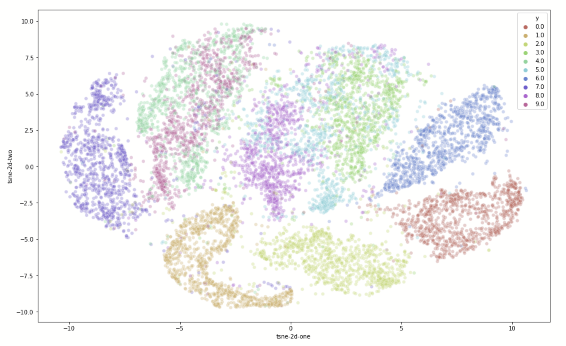
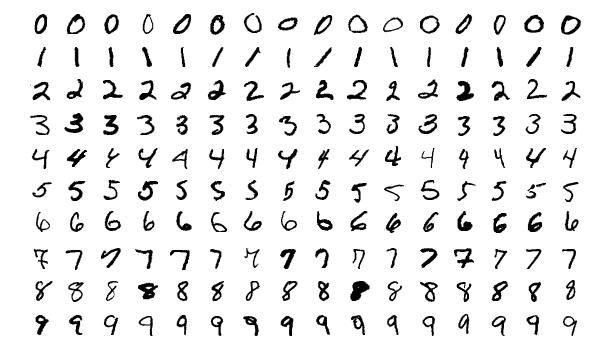
- MNIST
- Reducing dimensions for visualization (t-SNE)
- From towardsdatascience.com
- From 28x28 dimensions to 2, with \(10^5\) samples
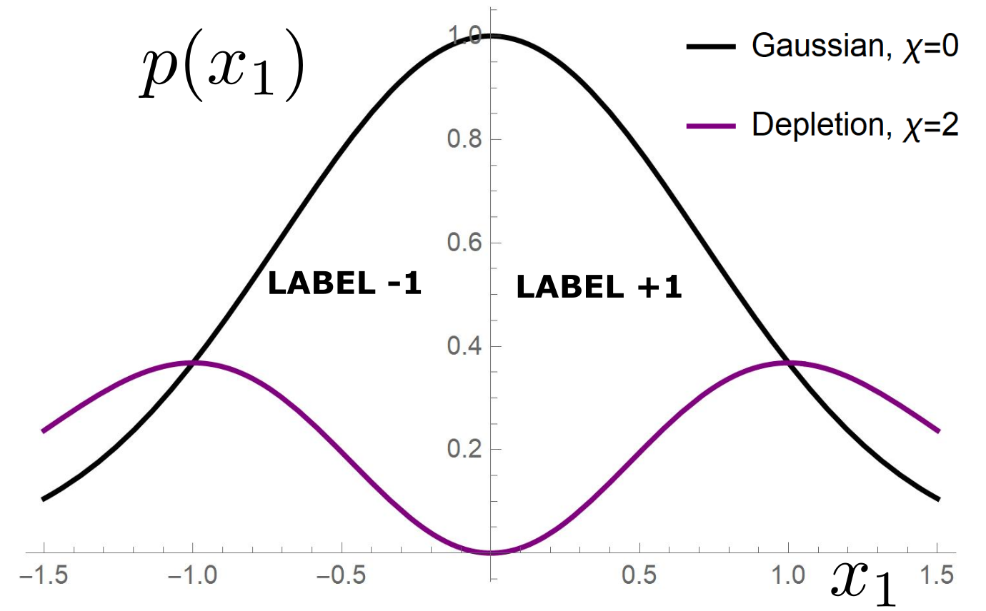
Depleted Stripe Model
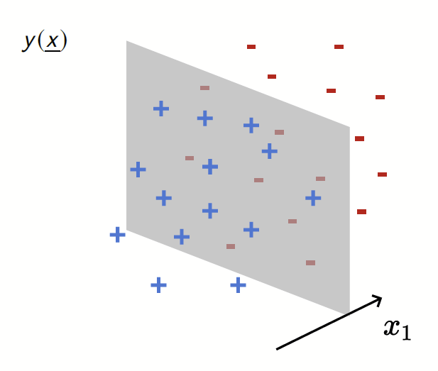
[Paccolat, Spigler, Wyart 2020]
Data: isotropic Gaussian
Label: \(f^*(x_1,x_{\bot})=\text{sign}[x_1]\)
Depletion of points around the interface
p(x_1)= \frac{1}{\mathcal{Z}}|x_1|^\chi e^{-x_1^2}
[Tomasini, Sclocchi, Wyart 2022]
Simple models: testing the KRR literature theories
- Based on replica theory, they predict the test error
- In the limit of \(\lambda\rightarrow 0^+\): spectral bias
- They work very well on real data. Yet, their validity limit is not clear;
- Which are the real data features which allow their success?
[Canatar et al., Nature (2021)]
KRR learns the first \(P\) eigenmodes of \(K\)
Test error: 2 regimes
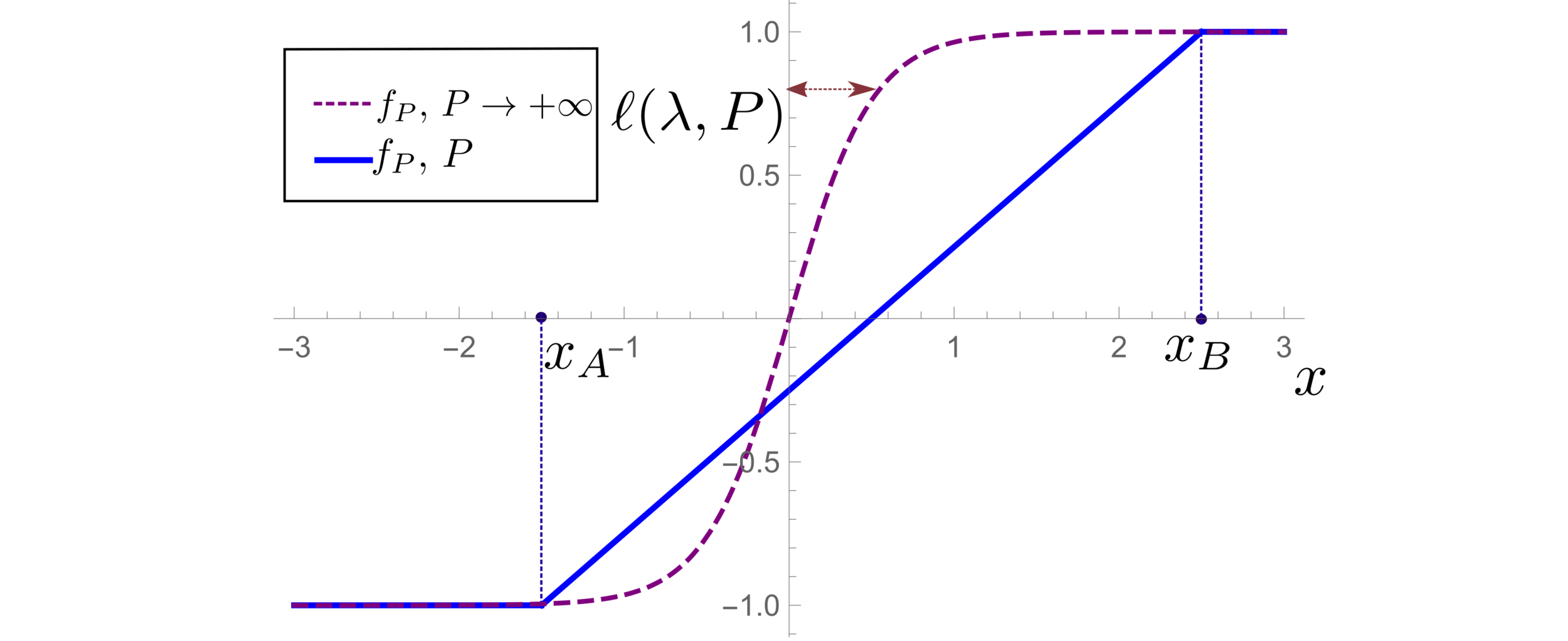
(1) For \(P\rightarrow \infty\): predictor controlled by characteristic length:
\( \ell(\lambda,P) \sim \left(\frac{ \lambda \sigma}{P}\right)^{\frac{1}{1+d+\chi}}\)
In this regime, replica prediction works.
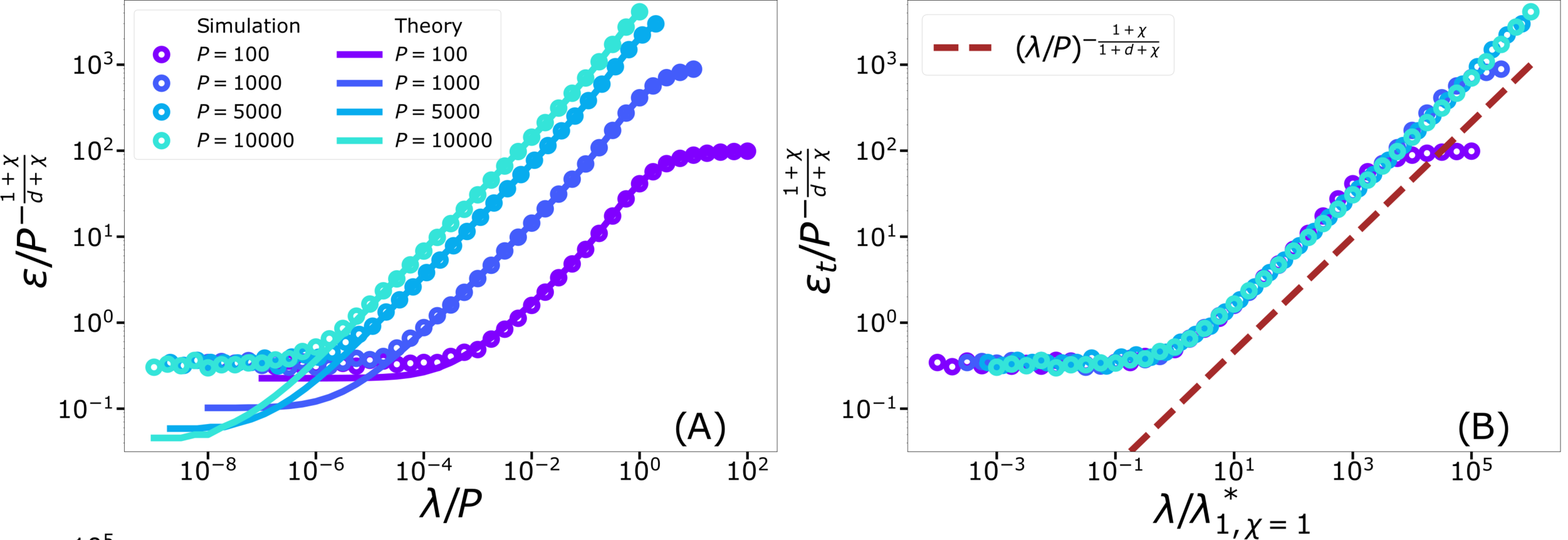
For fixed regularizer \(\lambda/P\):
Test error: 2 regimes
For fixed regularizer \(\lambda/P\):
\(\rightarrow\) Predictor controlled by extreme value statistics of \(x_B\)
\(\rightarrow\) Not self-averaging: no replica theory
(2) For small \(P\): predictor controlled by extremal sampled points:
\(x_B\sim P^{-\frac{1}{\chi+d}}\)
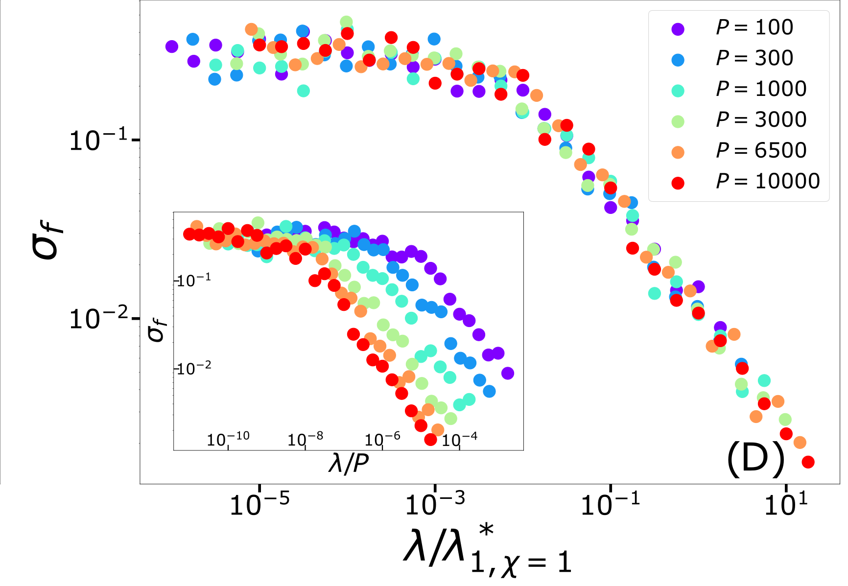
The self-averageness crossover
\(\rightarrow\) Comparing the two characteristic lengths \(\ell(\lambda,P)\) and \(x_B\):
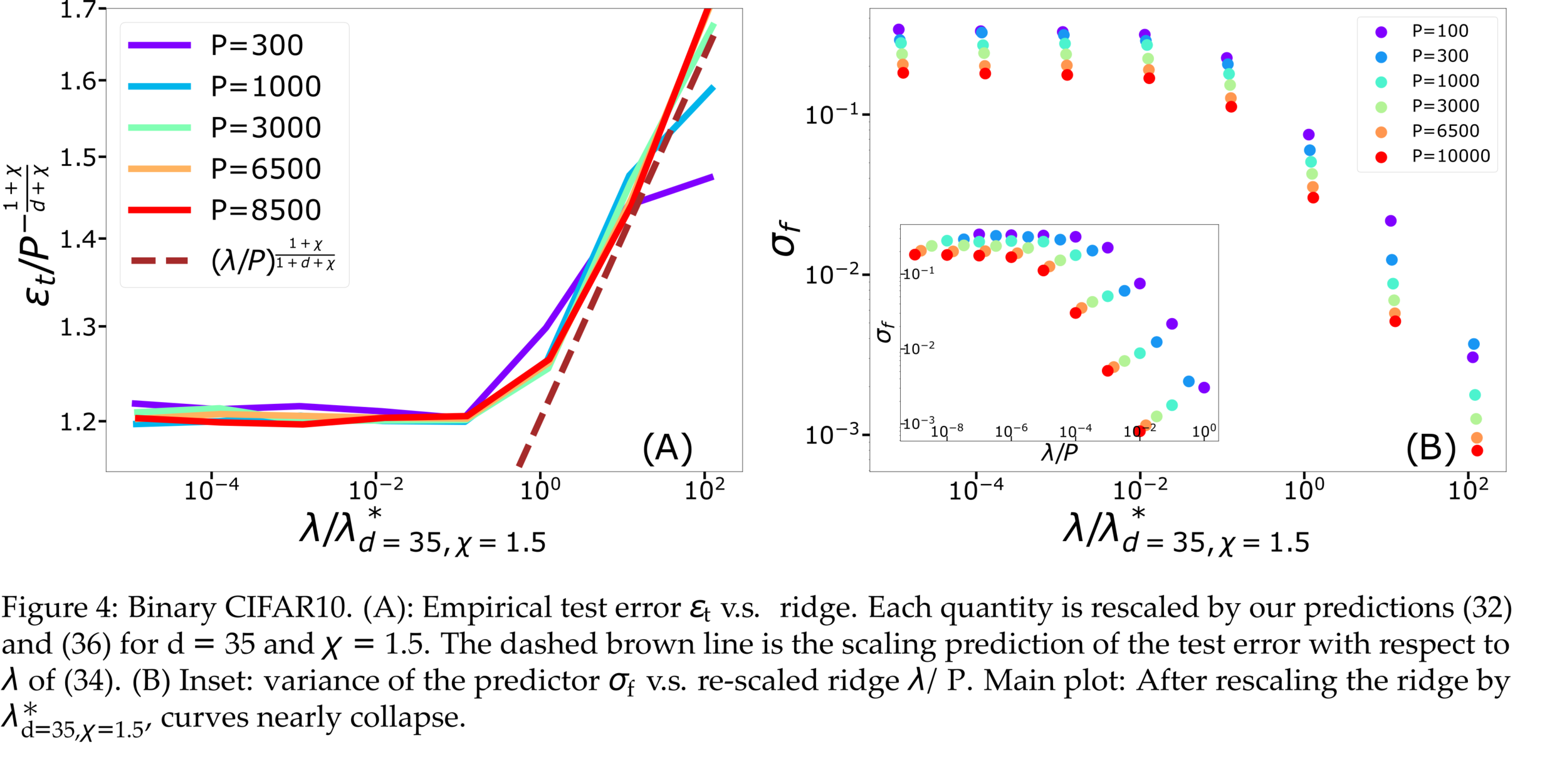
\lambda^*_{d,\chi}\sim P^{-\frac{1}{d+\chi}}
\sigma_f = \langle [f_{P,1}(x_i) - f_{P,2}(x_i)]^2 \rangle
\varepsilon_B \sim P^{-(1+\frac{1}{d})\frac{1+\chi}{1+d+\chi}}
\varepsilon_t \sim P^{-\frac{1+\chi}{d+\chi}}
\neq
Different predictions for
\(\lambda\rightarrow0^+\)
- For \(\chi=0\): equal
- For \(\chi>0\): equal for \(d\rightarrow\infty\)
Conclusions
- Replica predictions works even for small \(d\), for large ridge.
- For small ridge: spectral bias prediction, if \(\chi>0\) correct just for \(d\rightarrow\infty\).
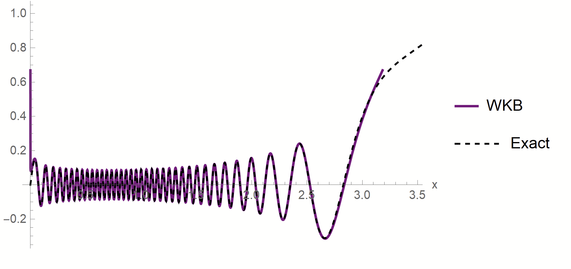
- To test spectral bias, we solved eigendecomposition of Laplacian kernel for non-uniform data, using quantum mechanics techniques (WKB).
- Spectral bias prediction based on Gaussian approximation: here we are out of Gaussian universality class.
Technical remarks:
Thank you for your attention.
BACKUP SLIDES
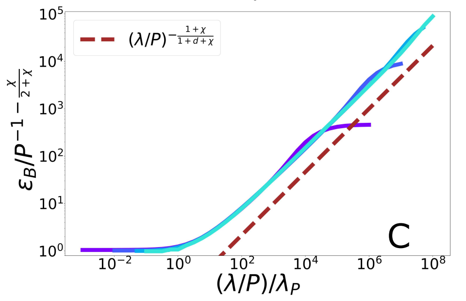
Scaling Spectral Bias prediction
Fitting CIFAR10
Proof:
- WKB approximation of \(\phi_\rho\) in [\(x_1^*,\,x_2^*\)]:
\(\phi_\rho(x)\sim \frac{1}{p(x)^{1/4}}\left[\alpha\sin\left(\frac{1}{\sqrt{\lambda_\rho}}\int^{x}p^{1/2}(z)dx\right)+\beta \cos\left(\frac{1}{\sqrt{\lambda_\rho}}\int^{x}p^{1/2}(z)dx\right)\right]\)
x_1^*
x_2^*
- MAF approximation outside [\(x_1^*,\,x_2^*\)]
\(x_1*\sim \lambda_\rho^{\frac{1}{\chi+2}}\)
\(x_2*\sim (-\log\lambda_\rho)^{1/2}\)
- WKB contribution to \(c_\rho\) is dominant in \(\lambda_\rho\)
- Main source WKB contribution:
first oscillations
Formal proof:
- Take training points \(x_1<...<x_P\)
- Find the predictor in \([x_i,x_{i+1}]\)
- Estimate contribute \(\varepsilon_i\) to \(\varepsilon_t\)
- Sum all the \(\varepsilon_i\)
Characteristic scale of predictor \(f_P\), \(d=1\)
\sigma^2 \partial_x^2 f_P(x) =\left(\frac{\sigma}{\lambda/P}p(x)+1\right)f_P(x)-\frac{\sigma}{\lambda/P}p(x)f^*(x)
Minimizing the train loss for \(P \rightarrow \infty\):
\(\rightarrow\) A non-homogeneous Schroedinger-like differential equation
\(\rightarrow\) Its solution yields:
\ell(\lambda,P)\sim \left(\frac{\lambda\sigma}{P}\right)^{\frac{1}{(2+\chi)}}
Characteristic scale of predictor \(f_P\), \(d>1\)
- Let's consider the predictor \(f_P\) minimizing the train loss for \(P \rightarrow \infty\).
f_P(x)=\int d^d\eta \frac{p(\eta) f^*(\eta)}{\lambda/P} G(x,\eta)
- With the Green function \(G\) satisfying:
\int d^dy K^{-1}(x-y) G_{\eta}(y) = \frac{p(x)}{\lambda/P} G_{\eta}(x) + \delta(x-\eta)
- In Fourier space:
\mathcal{F}[K](q)^{-1} \mathcal{F}[G_{\eta}](q) = \frac{1}{\lambda/P} \mathcal{F}[p\ G_{\eta}](q) + e^{-i q \eta}
- In Fourier space:
\mathcal{F}[K](q)^{-1} \mathcal{F}[G_{\eta}](q) = \frac{1}{\lambda/P} \mathcal{F}[p\ G_{\eta}](q) + e^{-i q \eta}
\begin{aligned}
\mathcal{F}[G](q)&\sim q^{-1-d}\ \ \ \text{for}\ \ \ q\gg q_c\\
\mathcal{F}[G](q)&\sim \frac{\lambda}{P}q^\chi\ \ \ \text{for}\ \ \ q\ll q_c\\
\text{with}\ \ \ q_C&\sim \left(\frac{\lambda}{P}\right)^{-\frac{1}{1+d+\chi}}
\end{aligned}
- Two regimes:
- \(G_\eta(x)\) has a scale:
\ell(\lambda,P)\sim 1/q_c\sim \left(\frac{\lambda}{P}\right)^{\frac{1}{1+d+\chi}}
Copy of VeniceTalk_WorkshopPoD
By umberto_tomasini


