Properties of equilibria and glassy phases of the random Lotka-Volterra model with demographic noise
Authors:
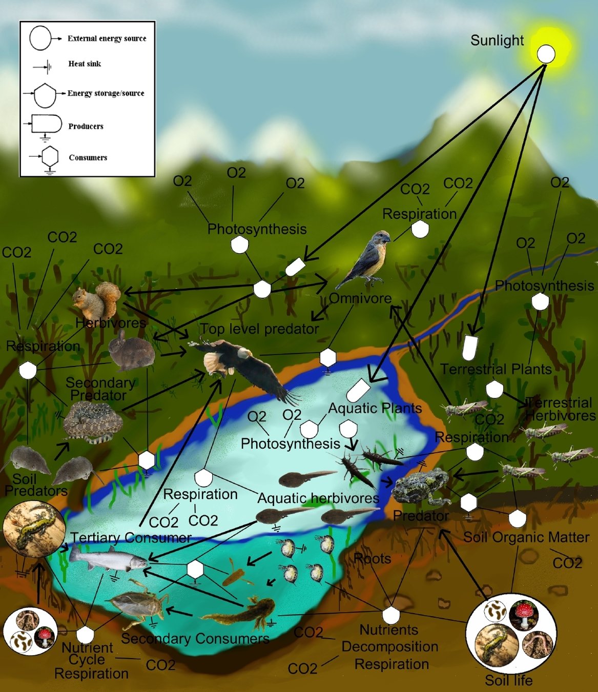
Ecosystems:
building blocks Nature
living species + environment
-
Short-time interactions:
- Predation (+,-)
-
Long-time interactions:
- Mutualism: (+,+)
- Commensalism: (0,+)
- Parassitism: (+,-)
- Competition (-,-)


Ecosystems are complex systems
Small number of species
-->Dynamical systems
Example: Lotka-Volterra for prey-predator system
\frac{dx}{dt} = \alpha x - \beta xy, \qquad \frac{dy}{dt} = -\gamma y + \delta xy

And for very large number of interacting species?
- Collective behaviours
- Statistical Physics well-suited
A model for well-mixed ecosystems:
disordered Lotka-Volterra model
\frac{dN_i}{dt} = N_i\left[1-N_i-\sum\limits_{j\neq i}\alpha_{ij}N_j\right]+\eta_i(t)
\(i\in\{1,...,S\}\)
- \(N_i\) exp growth term
- \(1-N_i\) accounts for limited resources
A model for well-mixed ecosystems:
disordered Lotka-Volterra model
\frac{dN_i}{dt} = N_i\left[1-N_i-\sum\limits_{j\neq i}\alpha_{ij}N_j\right]+\eta_i(t)
\(i\in\{1,...,S\}\)
Symmetric interaction matrix
- mean[\(\alpha_{ij}\)]=\(\frac{\mu}{S}\)
- var[\(\alpha_{ij}\)]=\(\frac{\sigma^2}{S}\)
- \(\alpha_{ij}=\alpha_{ji}\)
A model for well-mixed ecosystems:
disordered Lotka-Volterra model
\frac{dN_i}{dt} = N_i\left[1-N_i-\sum\limits_{j\neq i}\alpha_{ij}N_j\right]+\eta_i(t)
\(i\in\{1,...,S\}\)
Demographic Noise
- Zero mean
- \(\langle\eta_i(t)\eta_j(t')\rangle=2TN_i\delta_{ij}\delta(t-t')\)
A model for well-mixed ecosystems:
disordered Lotka-Volterra model
\frac{dN_i}{dt} = N_i\left[1-N_i-\sum\limits_{j\neq i}\alpha_{ij}N_j\right]+\eta_i(t)+\textcolor{blue}{\lambda}
Immigration: Reflecting boundaries at \(\textcolor{blue}{N_i=\lambda}\)
At stationarity
P(\{N_i\})=\exp(-\frac{H(\{N_i\})}{T})
\begin{aligned}
H = -\sum\limits_i\left(N_i-\frac{1}{2}N_i^2\right)+\frac{1}{2}\sum\limits_{i\neq j}\alpha_{ij} N_i N_j+\\
+\sum\limits_i\left[T\log N_i-\log(\theta(N_i-\lambda))\right]
\end{aligned}
How many equilibria?
A replica approach
-\beta F= \lim\limits_{n\rightarrow 0}\frac{\log\overline{Z^n}}{n}
\overline{Z^n}=\overline{\Pi_a \int \Pi_i dN_i^a e^{\left[-\beta H(\{N_i^a\})\right]}}
\overline{Z^n}=\int \Pi_{a,b} dQ_{ab}dQ_{aa}dH_{a}e^{S\mathcal{A}(Q_{ab},Q_{aa},H_{a})}
\(Q_{ab}=\frac{1}{S}\sum\limits^S\limits_{i=1} N_i^a N_i^b\)
\(H_{a}=\frac{1}{S}\sum\limits^S\limits_{i=1} N_i^a \)
Order Parameters:
\(\beta=\frac{1}{T}\)
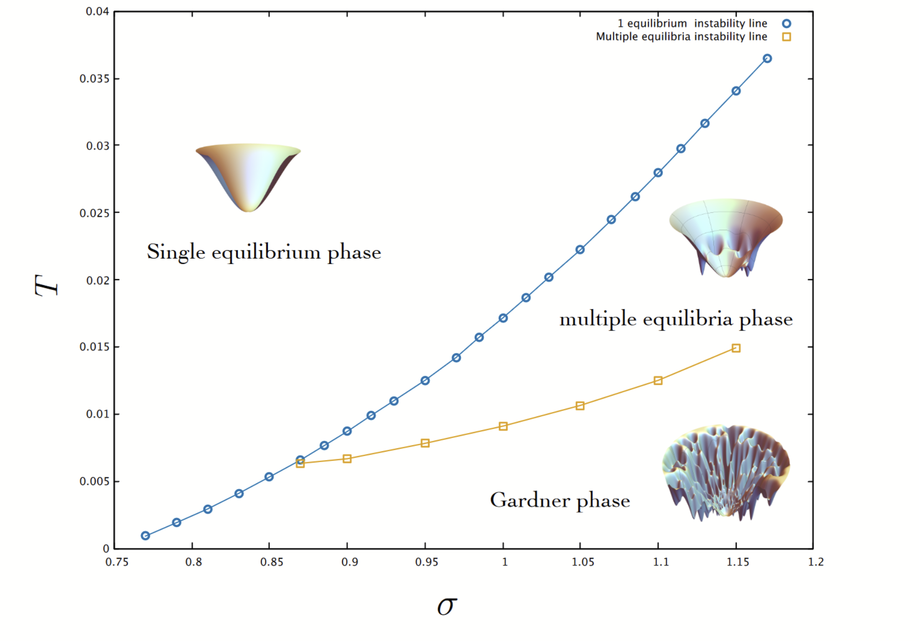
Phase Diagram
\(\lambda=0.01\) and \(\mu=10\)
Large \(T\):
- One equilibrium
- Noise \(\gg\) interactions
Obtained through a Replica Symmetry (RS) ansatz for Q
Phase transition lowering \(T\)
\mathcal{M}_{abcd}=-\frac{\mathcal{A}(Q_{ab},Q_{aa},H_{a})}{\partial Q_{ab}\partial Q_{cd}}
Lowering \(T\), the smallest eigenvalue \(\lambda_R\) of \(\mathcal{M}\) goes to 0
\(\lambda_R=(\beta\sigma)^2\left[1-(\beta\sigma)^2\overline{(\langle N_i^2\rangle-\langle N_i\rangle^2)^2}\right]=0\)
Phase Diagram
\(\lambda=0.01\) and \(\mu=10\)
- Exponential number of equilibria
- Interactions play a role
Obtained through a 1-Replica Symmetry Breaking (1RSB) ansatz for Q
Phase Diagram
\(\lambda=0.01\) and \(\mu=10\)
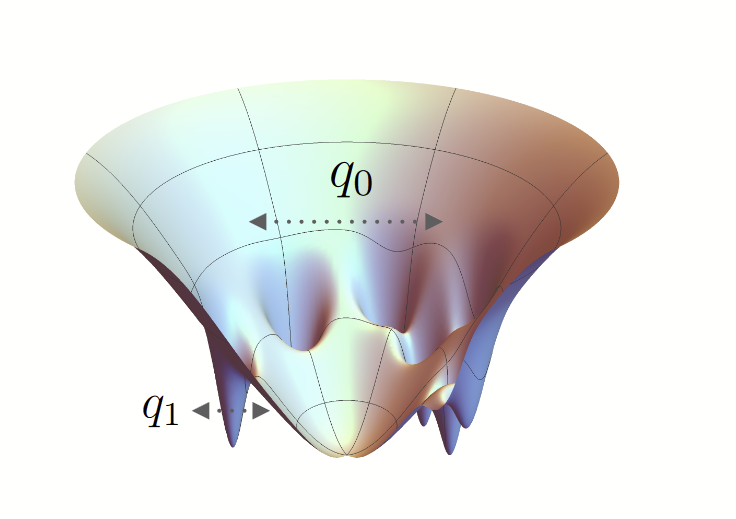
Gardner Phase
- Each equilibrium: many marginally-stable equilibria
- Fractal structure
One equilibrium Phase: dynamics
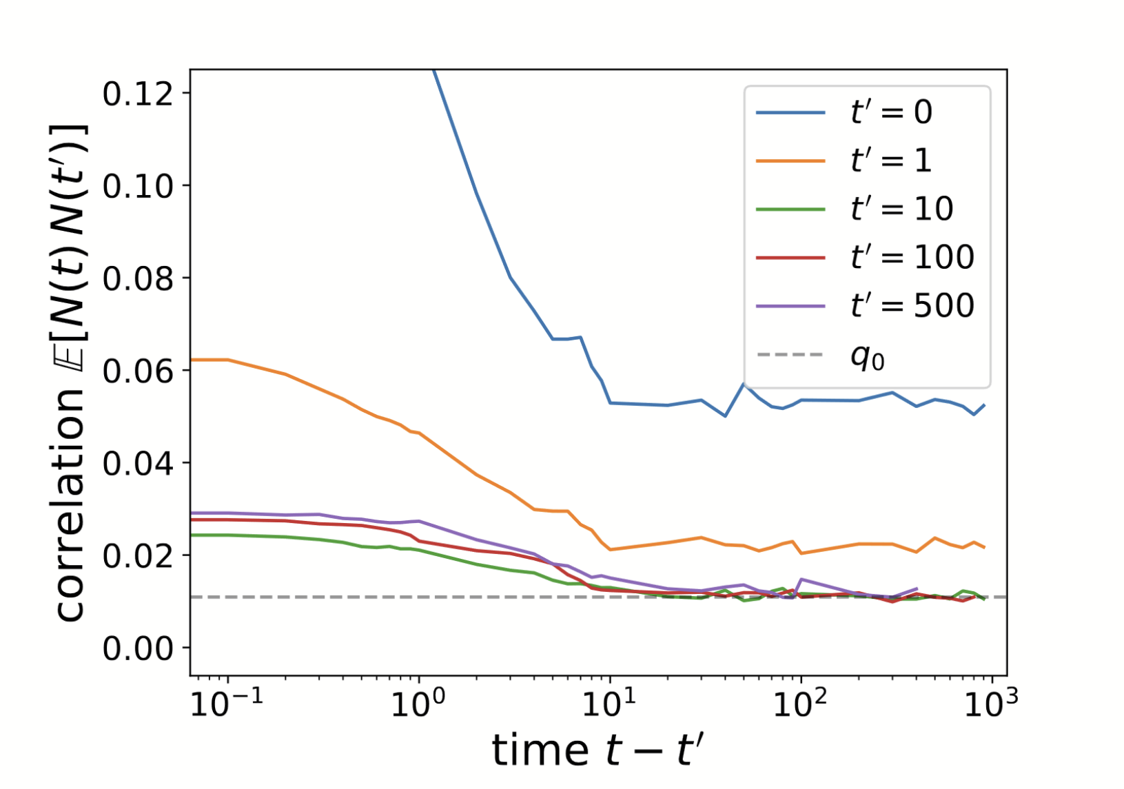
\(C(t,t')=\mathbb{E}[N(t)N(t')]=\frac{1}{S}\sum\limits_{i=1}^S\frac{1}{N_{sample}}\sum_{r=1}^{N_{sample}}N_i^r(t)N_i^r(t')\)
\(C(t,t')\approx C(t-t')\)
\((S,\mu,\sigma,\lambda,T)=(500,10,1,10^{-2},10^{-1})\)
Approaching the multi-equilibria Phase Transition
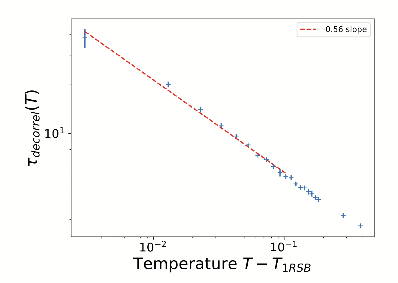
\((S,\mu,\sigma,\lambda)=(500,10,1,10^{-2})\)
\(\frac{C(\tau_{decorell})-C(\infty)}{C(0)-C(\infty)}=0.3\)
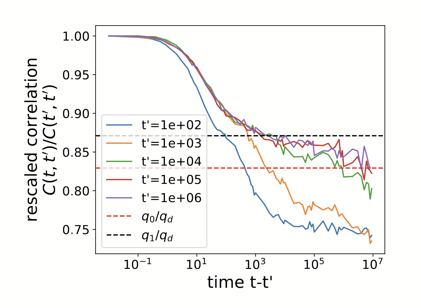
Aging in multiple equilibria phase
\((S,\mu,\sigma,\lambda,T)=(2000,10,1,10^{-2},1/80)\)
Hopping on metastable equilibria
Ecosystems: marginally stable?
\frac{dN}{dt}=b-\frac{N}{\tau}+\sqrt{D\,N}\xi(t)
\langle\xi(t)\xi(t')\rangle=2\delta(t-t')
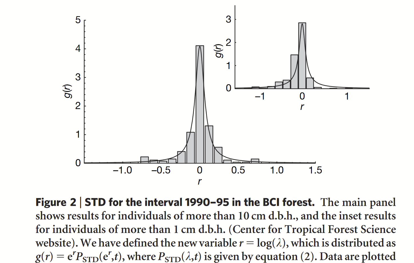
Fitting with Data
Stationarity: \(P_{st}(N)\)
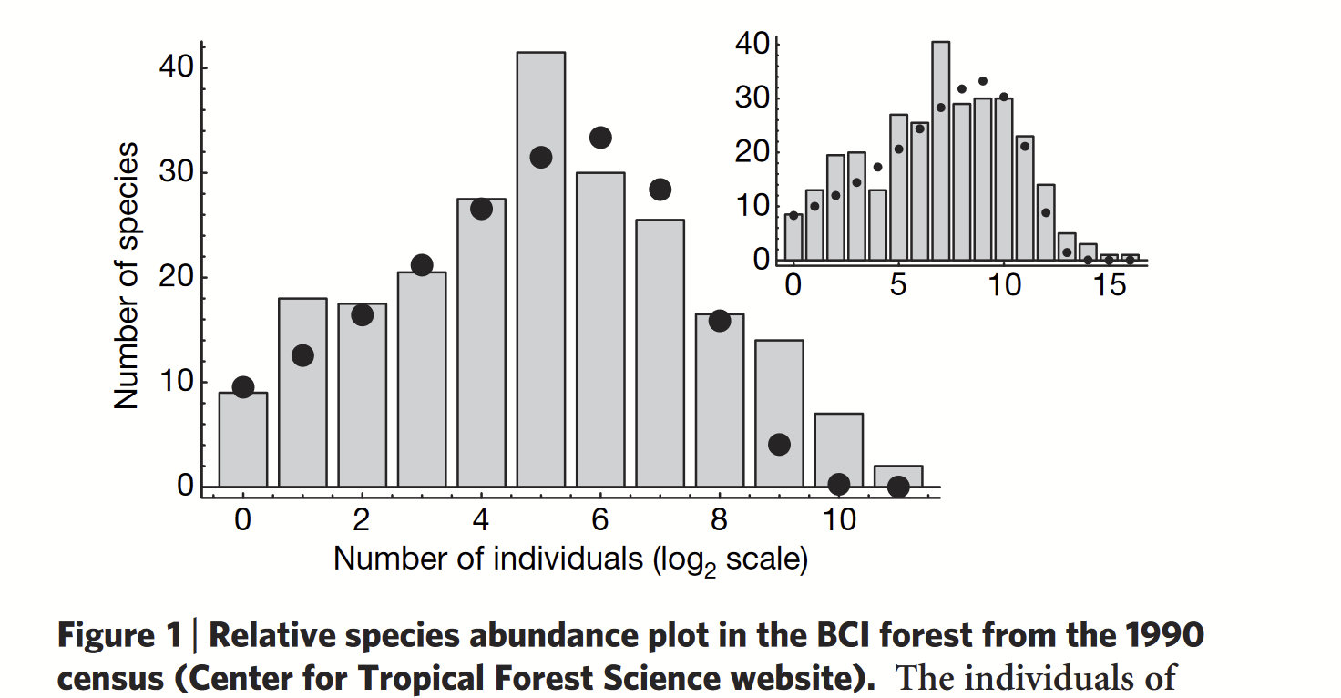
Time-dependent: \(P(\lambda, t)=P(\frac{N(t)}{N(0)},t)\)
Parameters estimation-> marginal stability
\begin{aligned}
b&=0.02\pm0.01\\
D&=0.04\pm0.02\\
\tau &= 3500\pm 1000\,\, years
\end{aligned}
\Rightarrow \langle t\rangle =\tau\left[\gamma-\frac{\Gamma'(1-b/D)}{\Gamma(1-b/D)}\right]\approx \tau
\gamma\approx 0.577
"Our result suggests that ecosystems at stationarity are marginally stable—not so stable that they are frozen in time and not so fragile that they are prone to extinction."
- \(\langle t\rangle\ll\tau\): extinction faster than recovery
- \(\langle t\rangle\gg\tau\): very robust ecosystem, no evolution
Where we are in the phase diagram?
- Obtain prediction for measurable ecological quantities
- Extrapolation of \(T,\sigma,\mu\)
Conclusions and questions
- Phase Diagram for random LV
- Small \(T\) and large \(\sigma\): many marginally stable equilibria
- Which is the phase for real ecosystems?
- Useful to understand what happens perturbing the ecosystem
- A question: response functions in glassy systems?
Thank you for your attention
BACKUP
Phase transition lowering \(T\)
from 1RSB to Gardner Phase
\mathcal{M}_{abcd}=-\frac{\mathcal{A}(Q_{ab},Q_{aa},H_{a})}{\partial Q_{ab}\partial Q_{cd}}
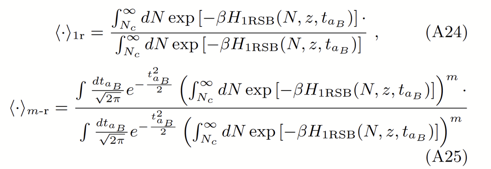
\(\lambda_R^{1rsb}=(\beta\sigma)^2\left[1-(\beta\sigma)^2\overline{\langle(\langle N^2\rangle_{1r}-\langle N_i\rangle_{1r}^2)^2\rangle_{m-r}}\right]=0\)
P(N)=\frac{(D\tau)^{-b/D}}{\Gamma(b/D)}N^{b/D-1}e^{-\frac{N}{D\tau}}
\begin{aligned}
P(\lambda,t)=A\frac{\lambda+1}{\lambda}\frac{(e^{t/\tau})^{b/2D}}{1-e^{-t/\tau}}\left(\frac{\sinh(t/2\tau)}{\lambda}\right)^{b/D-1}\\
\left(\frac{4\lambda^2}{(\lambda+1)^2e^{t/\tau}}-4\lambda\right)^{b/D+1/2}
\end{aligned}
\(\lambda=\frac{N(t)}{N(0)}\)
Properties of equilibria and glassy phases of the random Lotka-Volterra model with demographic noise
By umberto_tomasini


