How Data Structures affect Generalization in Kernel Methods and Deep Learning

Umberto Maria Tomasini
1/29
Public defense @
Failure and success of the spectral bias prediction for Laplace Kernel Ridge Regression: the case of low-dimensional data
UMT, Sclocchi, Wyart
ICML 22
How deep convolutional neural network
lose spatial information with training
UMT, Petrini, Cagnetta, Wyart
ICLR23 Workshop,
Machine Learning: Science and Technology 2023
How deep neural networks learn compositional data:
The random hierarchy model
Cagnetta, Petrini, UMT, Favero, Wyart
PRX 24
How Deep Networks Learn Sparse and Hierarchical Data:
the Sparse Random Hierarchy Model
UMT, Wyart
ICML 24
Clusterized data
Invariance to deformations
Invariance to deformations
Hierarchy
Hierarchy
2/29
Introduction: what is Machine Learning
-
Humans perform certain tasks almost automatically with enough skill and expertise
- Examples: driving, understand other languages, distinguish animal species, tumors in medical images, planning


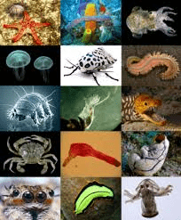
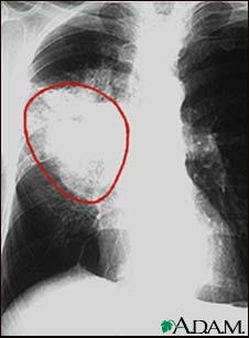

- Machines can learn and automatize tasks at scale
- Beyond human capability
- Too many data
- Too complex tasks
- When a machine has seen a lot of the world, it can become your wise friend, e.g. ChatGPT

3/29
How does Machine Learning work?

ML model
"Cat"
ML model
"Dog"
A simple task: classifying images based on whether they contain a cat or a dog
4/29
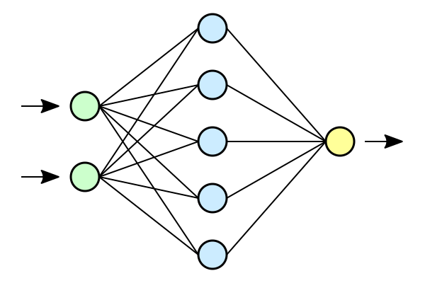
What there is inside the ML model?
"Dog"
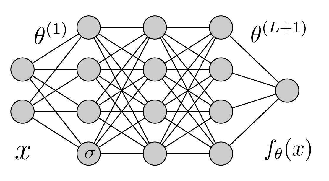
- Artificial Neurons
- Determining the ML model decision
- They learn to correctly classify images
5/29
ML models learn by examples
- Show labeled training examples to the ML model
- The neurons will adapt to classify correctly
"Cat"
"Dog"

- Repeat for thousands of images


6/29
Testing the trained model
on unseen images
"Cat"
"Dog"
- Test images: new, not used in training
- Quantify how good is the model:
- Percentage (%) of correct predictions
These models can be very good!
\(\rightarrow\) Surprising, images are difficult for a PC
7/29
76
76
76
76
76
76
76
76
76
76
76
76
76
76
76
92
92
92
27
27
27
27
27
27
27
27
27
27
27
27
27
27
27
27
27
27
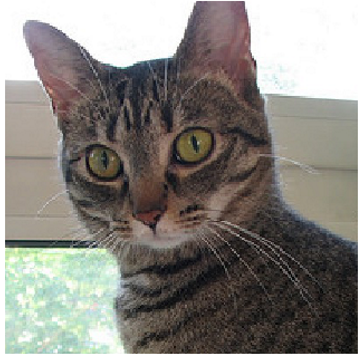
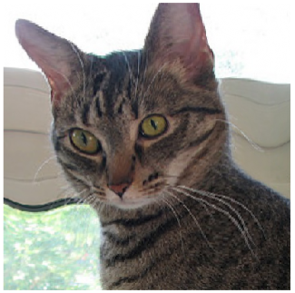
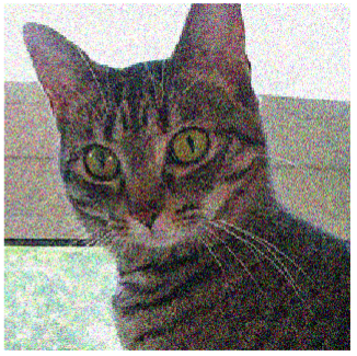
Hard to visualize. With a small change:
- Still a dog
- Very different pixels!
How can a ML model compare them?
27
27
27
27
27
27
27
27
27
27
27
27
27
27
27
27
27
27
27
27
27
27
27
27
27
27
27
27
27
27
27
27
27
27
27
27
How a computer sees an image
Pixels!
8/29
Learning to classify images
76
76
76
76
76
76
76
76
76
76
76
76
76
76
76
92
92
92
27
27
27
27
27
27
27
27
27
27
27
27
27
27
27
27
27
27
"Dog"
Goal: learning function that given \(d\) pixels, returns the correct label
Difficulty increases with \(d\)
[images idea by Leonardo Petrini]
\(d=2\)


\(d=1\)
\(d=3\)
9/29
The Curse of Dimensionality
- Images can be made by \(d=\) millions pixels
- Not representable
Simplest technique to learn:
- Just sample training points in this space and locally interpolate new test data
- Very inefficient: images are very distant in this space, for resolution \(\varepsilon\), a number of training points \(P\) exponential in \(d\) is required
\(P\propto (1/\varepsilon)^{d}\)
\(\Rightarrow\) Not the case for ML!
10/29
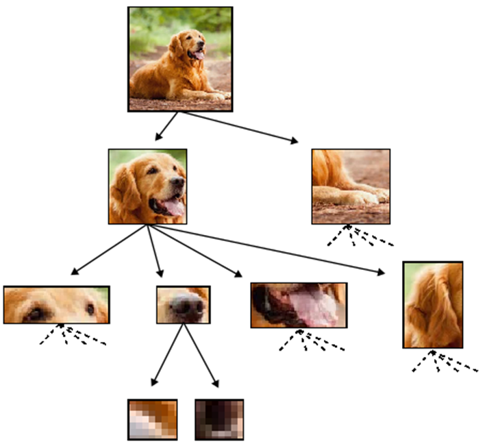
Humans Simplify and Understand
To classify a dog, we do not need every bit of information within the data.
- Locate the object
- Detect the components of the object
- Independently on their exact positions/realizations
Many irrelevant details that can be disregarded to solve the task.
- Recognizing the components, the meaning of the object can be inferred
- Accordingly to the structure of the dog
"Dog"

"Dog"
11/29
Key questions motivating this thesis:
- What constitutes a learnable structure ?
- How does Machine Learning exploit it?
- How many training points are required?
What about Machine Learning?
12/29
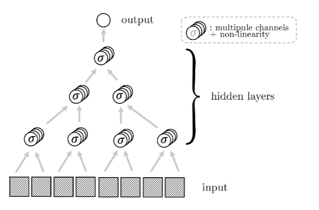
Reducing complexity with depth
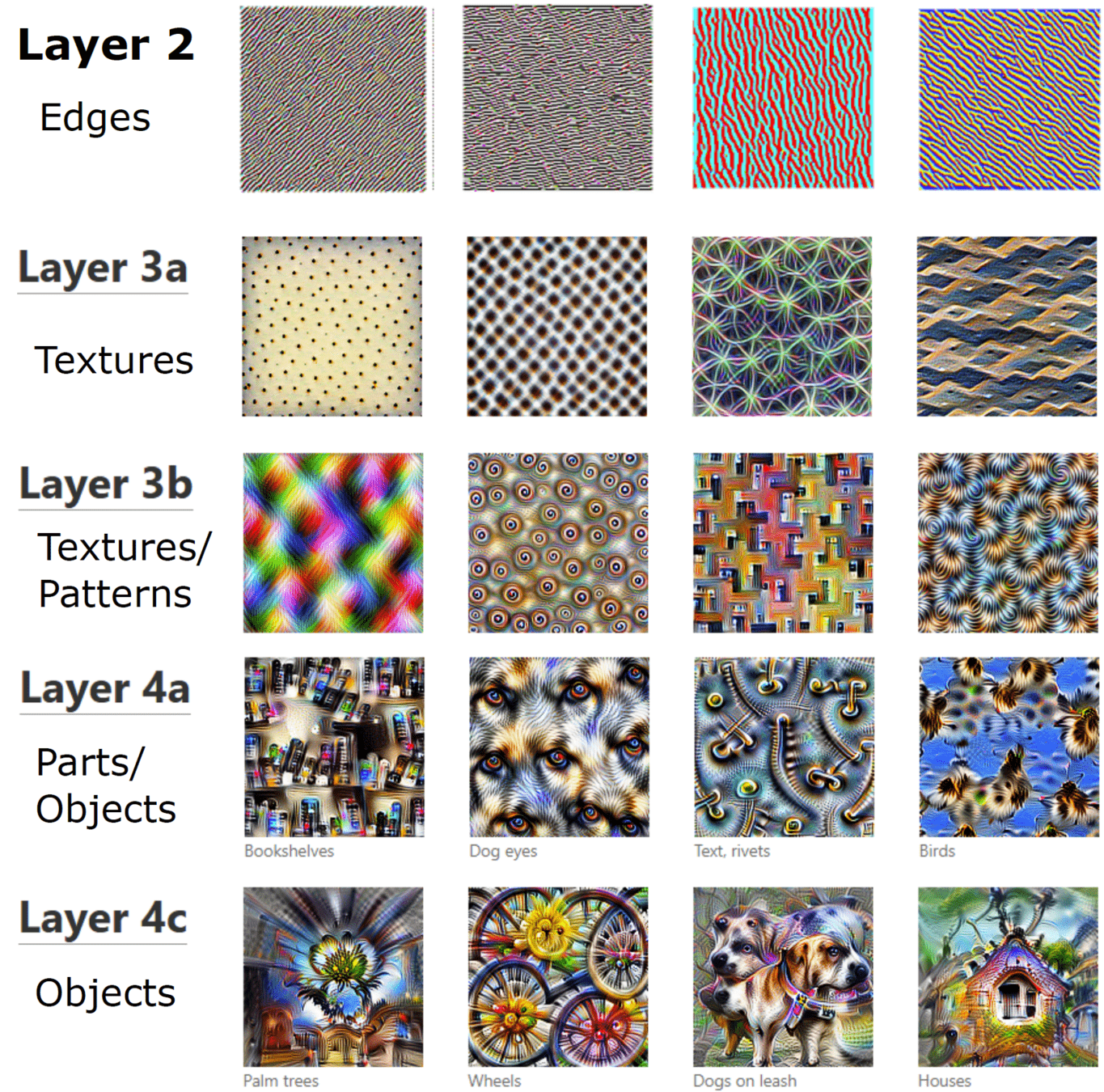
Deep networks build increasingly abstract representations with depth (also in brain)
- How many training points are needed?
- Why are these representations effective?
Intuition: reduces complexity of the task, ultimately beating curse of dimensionality.
- Which irrelevant information is lost ?
[Zeiler and Fergus 14, Yosinski 15, Olah 17, Doimo 20,
Van Essen 83, Grill-Spector 04]
[Shwartz-Ziv and Tishby 17, Ansuini 19, Recanatesi 19, ]
13/29
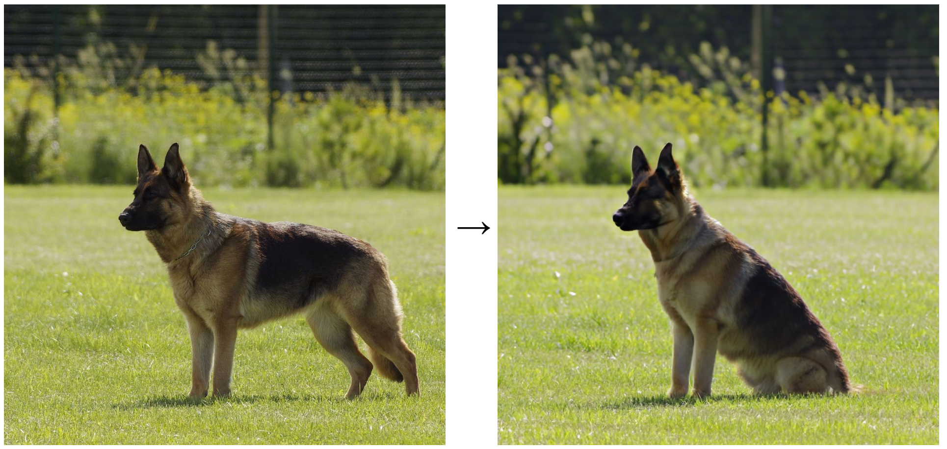
Two ways for ML to lose information
by learning invariances
Discrete
Continuous (diffeomorphisms
[Bruna and Mallat 13, Mallat 16, Petrini 21]
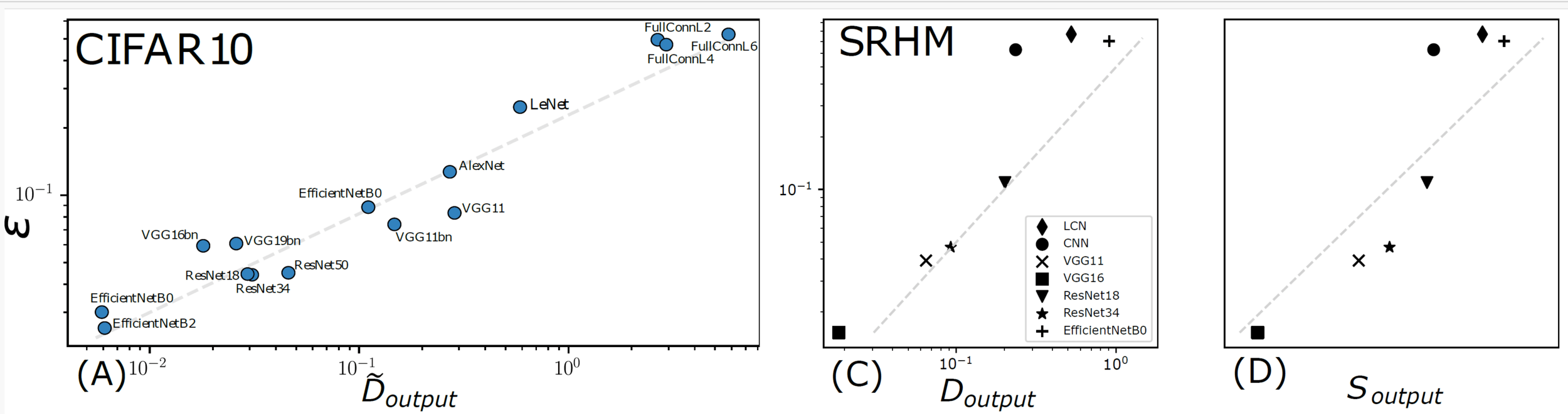
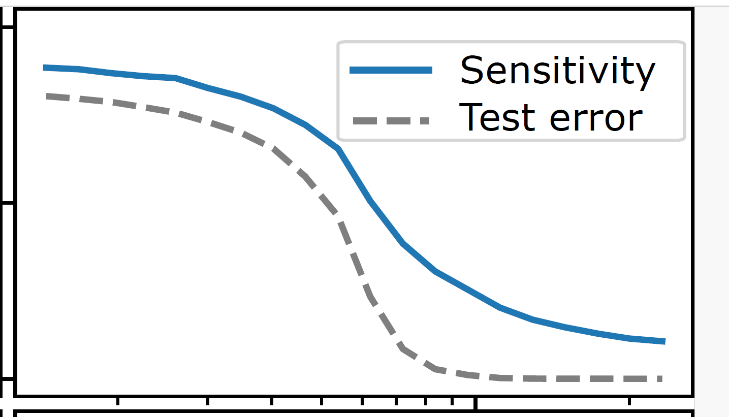
Test error correlates with sensitivity to diffeo
[Petrini21]
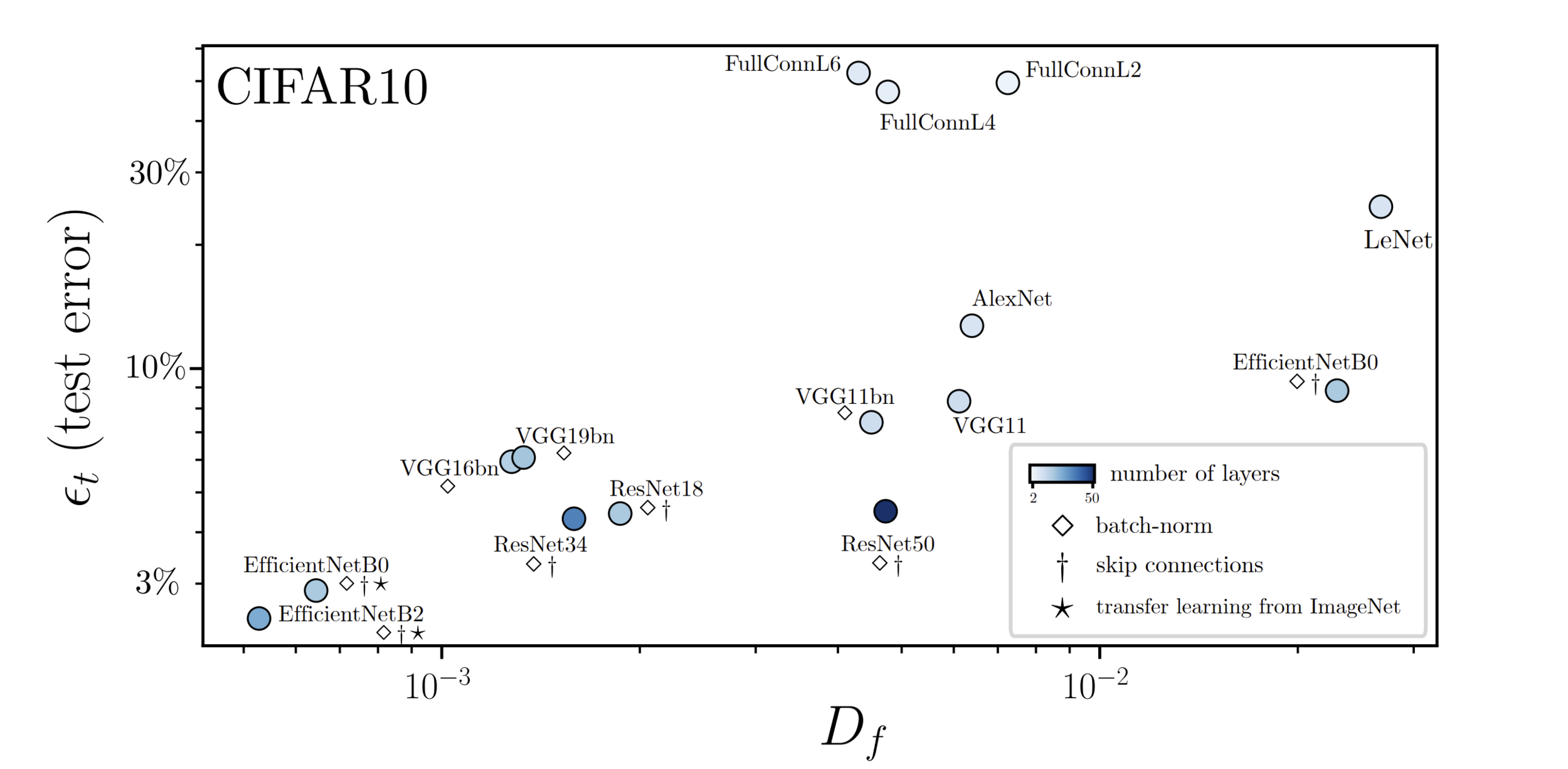
Sensitivity to diffeo
Test error
+Sensitive
14/29
- Compositional structure of data,
- Hierarchical structure of data,
This thesis:
data properties learnable by deep networks
[Poggio 17, Mossel 16, Malach 18-20, Schmdit-Hieber 20, Allen-Zhu and Li 24]
3. Data are sparse,
4. The task is stable to transformations.
[Bruna and Mallat 13, Mallat 16, Petrini 21]
How many training points are needed for deep networks?
15/29
Outline
Part I: introduce a hierarchical model of data to quantify the gain in number of training points.
Part II: understand why the best networks are the least sensitive to diffeo, in an extension of the hierarchical model.
16/29
Part I: Hierarchical structure
Do deep hierarchical representations exploit the hierarchical structure of data?
[Poggio 17, Mossel 16, Malach 18-20, Schmdit-Hieber 20, Allen-Zhu and Li 24]
How many training points?
Quantitative predictions in a model of data
[Cagnetta, Petrini, UMT, Favero, Wyart, PRX 24]
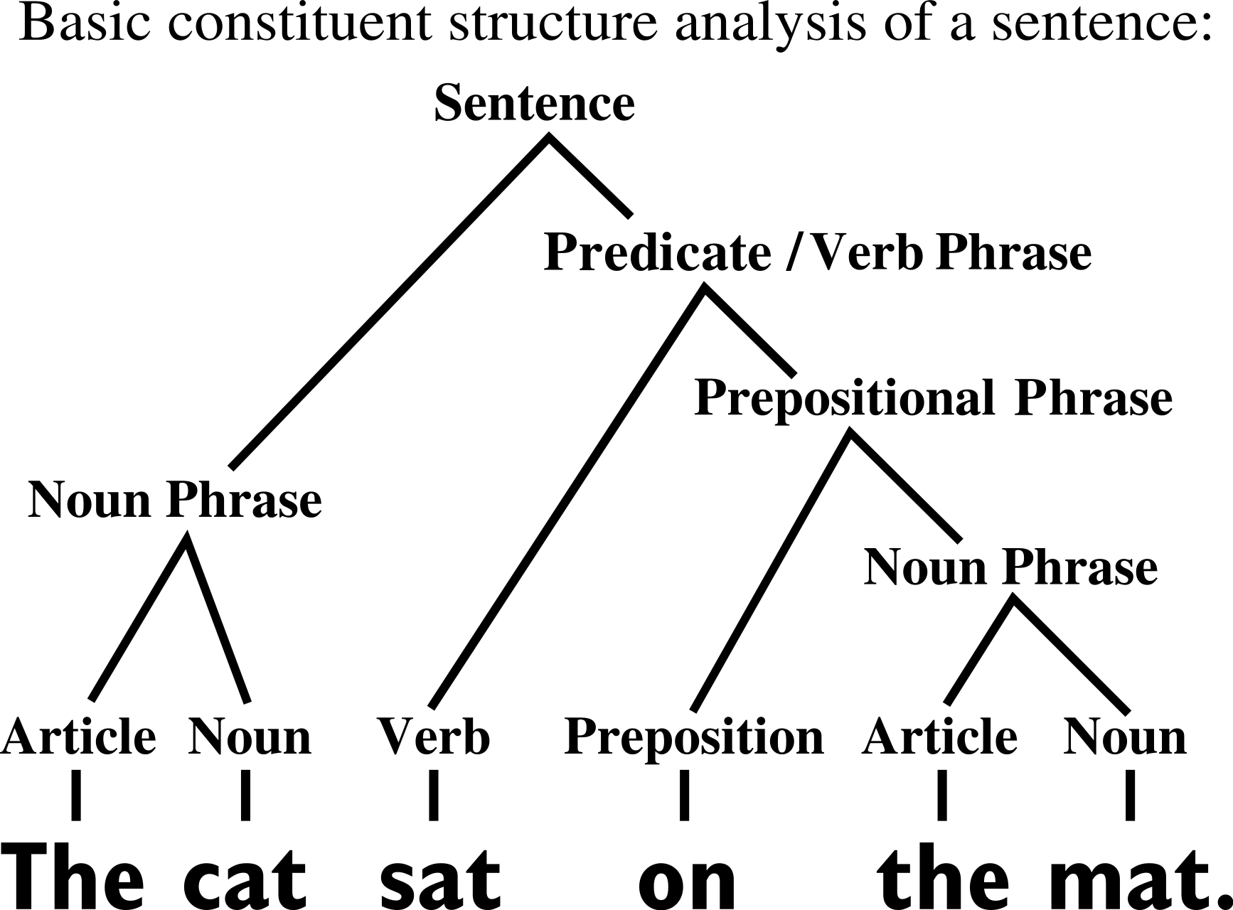
sofa
[Chomsky 1965]
[Grenander 1996]
17/29
Random Hierarchy Model
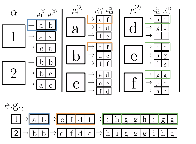
- Generative model: label generates a patch of \(s\) features, chosen from vocabulary of size \(v\)
- Patches chosen randomly from \(m\) different random choices, called synonyms
- Each label is represented by different patches (no overlap)
- Generation iterated \(L\) times with a fixed tree topology.
- Dimension input image: \(d=s^L\)
- Number of data: exponential in \(d\), memorization not practical.
18/29
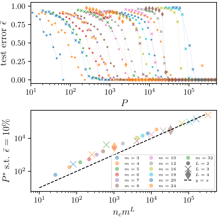
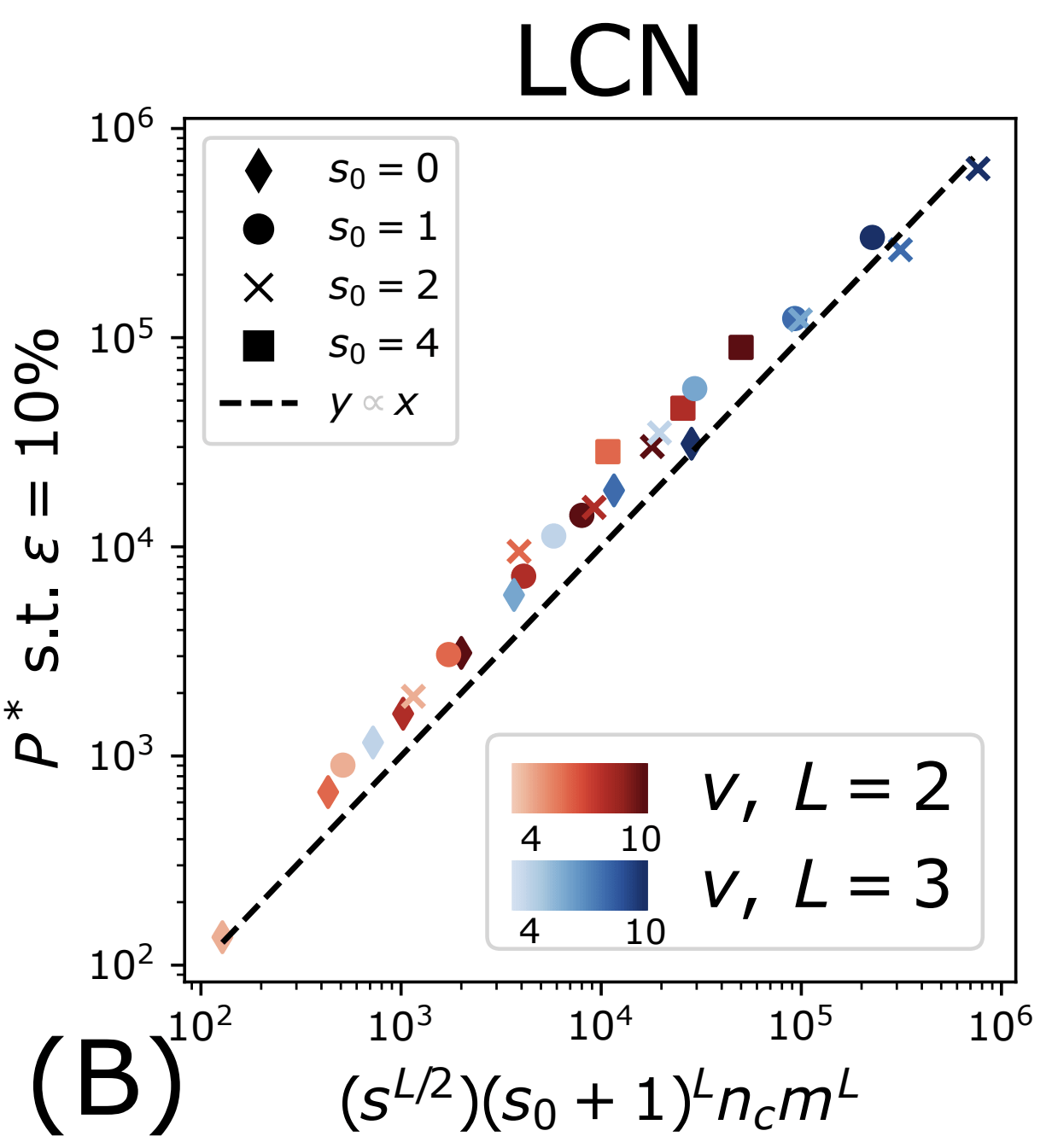
Deep networks beat the curse of dimensionality
\(P^*\)
\(P^*\sim n_c m^L\)
- Polynomial in the input dimension \(s^L\)
- Beating the curse
- Shallow network \(\rightarrow\) cursed by dimensionality
- Depth is key to beat the curse
19/29
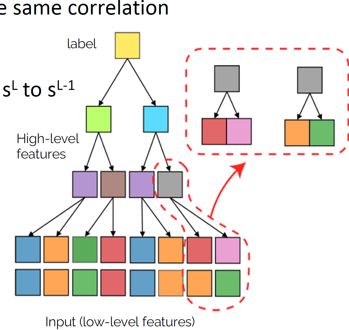
How deep networks learn the hierarchy?
- Intuition: build a hierarchical representation mirroring the hierarchical structure. How to build such representation?
- Start from the bottom. Group synonyms: learn that patches in input correspond to the same higher-level feature
- Collapse representations for synonyms, lowering dimension from \(s^L\) to \(s^{L-1}\)
- Iterate \(L\) times to get hierarchy
20/29
To group the synonyms, \(P^*\sim n_c m^L\) points are needed
Takeaways
- Deep networks learn hierarchical tasks with a number of data polynomial in the input dimension
- They do so by developing internal representations that learn the hierarchical structure layer by layer
Limitations
- To think about images, missing invariance to smooth transformations
- RHM is brittle: a spatial transformation changes the structure/label
Part II
- Extension of RHM to connect with images
- Useful to understand why good networks develop representations insensitive to diffeomorphisms
21/29
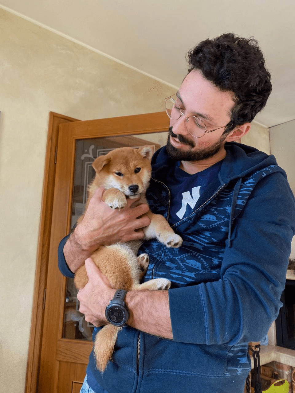
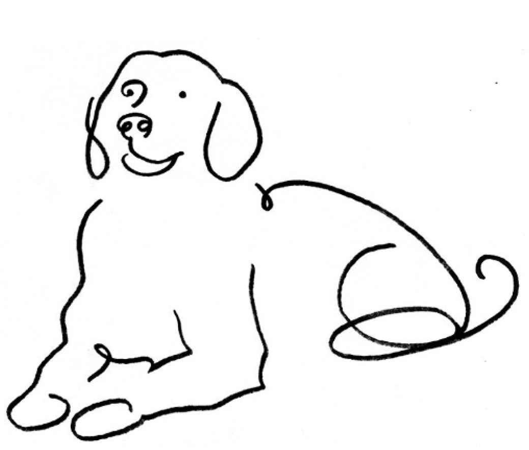
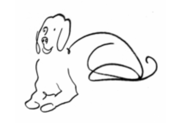
Key insight: sparsity brings invariance to diffeo
- Humans can classify images even from sketches
- Why? Images are made by local and sparse features.
- Their exact positions do not matter.
- \(\rightarrow\) invariance of the task to small local transformations, like diffeomorphisms.
- We incorporate this simple idea in a model of data
[Tomasini, Wyart, ICML 24]
22/29
Sparse Random Hierarchy Model
- Keeping the hierarchical structure
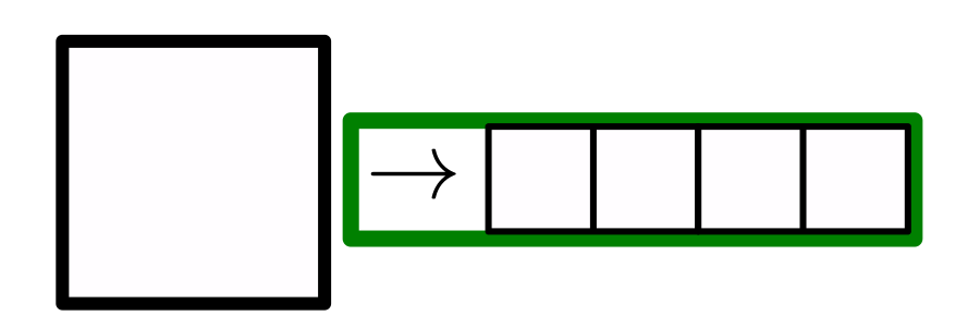
- Each feature is embedded in a sub-patch with \(s_0\) uninformative features.
- The uninformative features are in random positions.
- They generate just uninformative features
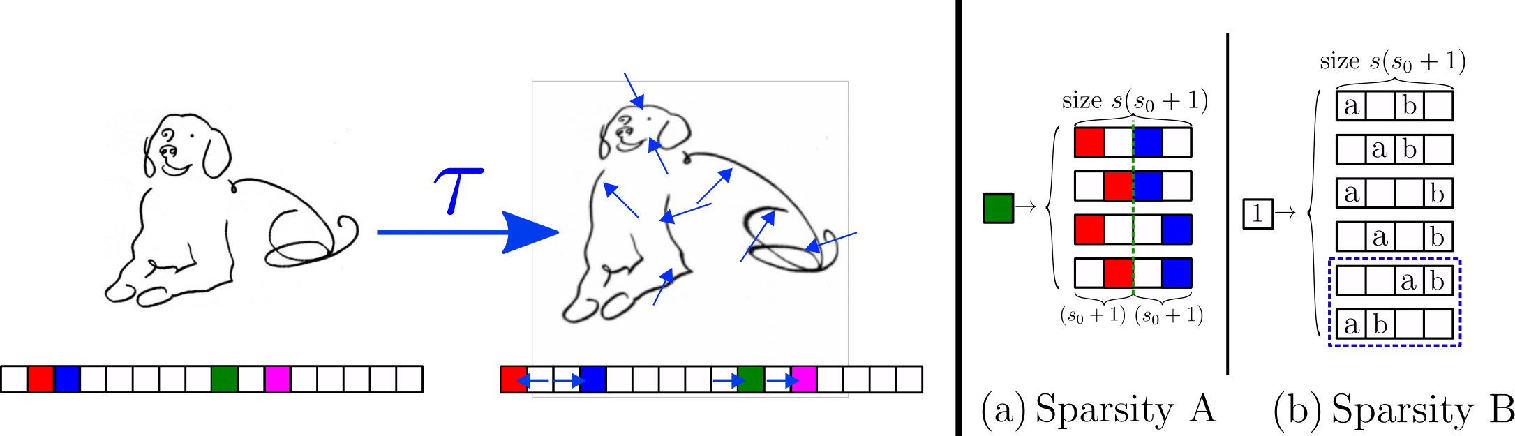
Sparsity\(\rightarrow\) Invariance to feature displacements (diffeo)
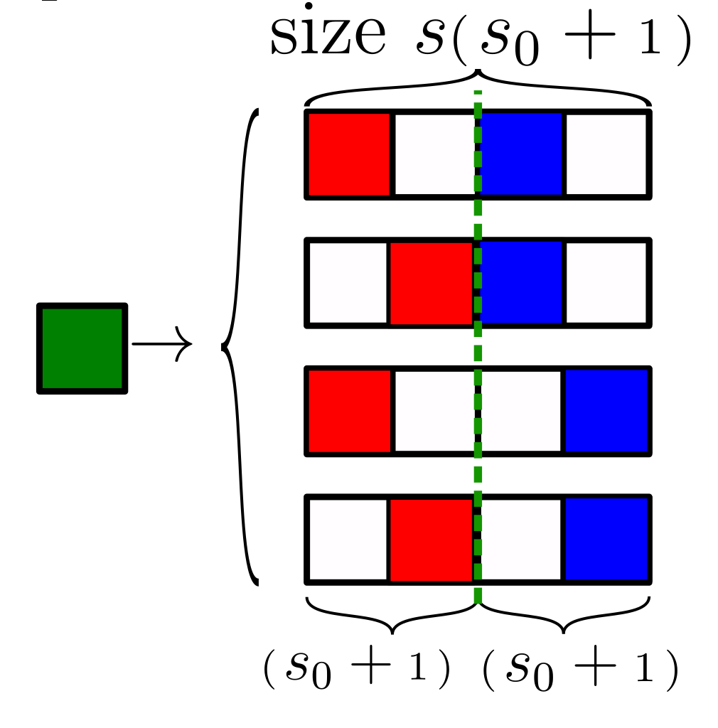
- Very sparse data, \(d=s^L(s_0+1)^L\)

Sparsity \(\rightarrow\) invariance to features displacements (diffeo)

23/29
Capturing correlation with performance
Analyzing this model:
- How many training points to learn the task?
- And to learn the insensitivity to diffeomorphisms?
Sensitivity to diffeo
Sensitivity to diffeo
Test error
24/29
Learning by detecting correlations
\(x_1\)
\(x_2\)
\(x_3\)
\(x_4\)
- Without sparsity: learning based on grouping synonyms.
- With sparsity: latent variables generate patches with synonyms, distorted with diffeo
- All these patches share the same correlation with the label.
- Such correlation can be used by the network to group patches when \(P>P^*\)
25/29
How many training points to detect correlations
- Without sparsity (\(s_0=0\)): \(P^*_0\)
-
With sparsity: to recover the synonyms, a factor \(1/p\) more data:
\(P^*_{\text{LCN}}\sim (1/p) P^*_0\)
- \(p\) depends on the ML architecture, still beating the curse
26/29
What happens to Representations?
- To see a local signal (correlations), \(P^*\) data are needed
- For \(P>P^*\), the local signal is seen in each location it may end up
- The representations become insensitive to the exact location: insensitivity to diffeomorphisms.
- At the same scale both synonyms and diffeo are learnt.
\(x_1\)
\(x_2\)
\(x_3\)
\(x_4\)
27/29
Takeaways
- Deep networks beat the curse of dimensionality on sparse hierarchical tasks.
- The hidden representations learn the hierarchical structure and to be invariant to spatial local transformations.
- The more insensitive the network is, the better is its performance.
28/29
The Bigger Picture
- How deep learning is able to solve high-dimensional tasks like image classification?
- We identified a few data structures that help the network to simplify and solve the problem
- The more we understand which are the relevant data structures, and the better ML models will be.
"Dog"
29/29
Thanks to the PCSL team!


Thanks to:

Thanks to:


Thanks to:


Thanks to:


Thanks to:


BACKUP SLIDES
Grouping synonyms by correlations
- Synonyms are patches with same correlation with the label
- Measure correlations by counting
- Large enough training set is required to overcome sampling noise:
- \(P^*\sim n_c m^L\), same as sample complexity
17/28
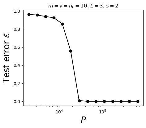
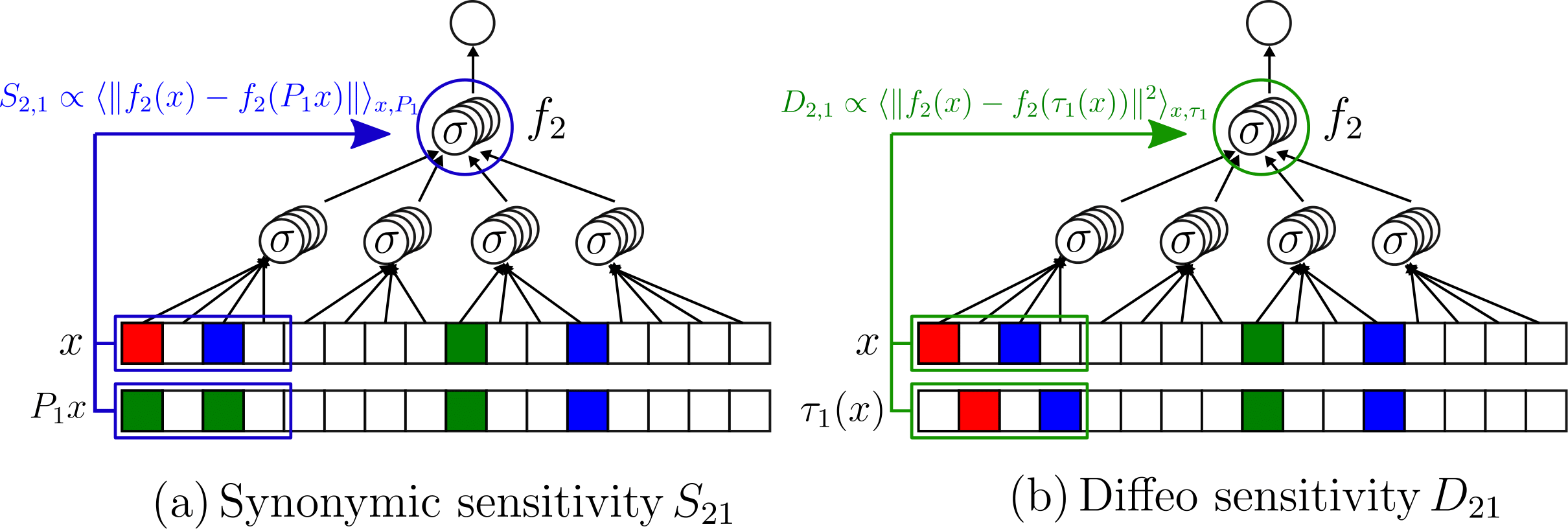
Testing whether deep representations collapse for synonyms
At \(P^*\) the task and the synonyms are learnt
- How much changing synonyms at first level in data change second layer representation (sensitivity)
- For \(P>P^*\) drops
1.0
0.5
0.0
\(10^4\)
Training set size \(P\)
18/28
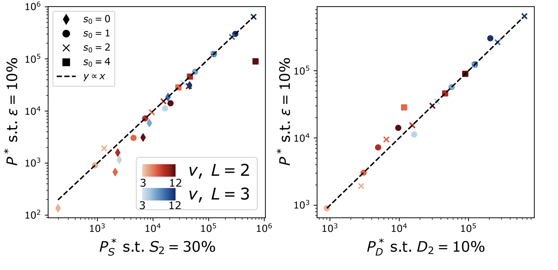
Learning both insensitivities at the same scale \(P^*\)
Diffeomorphisms
learnt with the task
Synonyms learnt with the task
The hidden representations become insensitive to the invariances of the task
26/28
More training leads to better performance
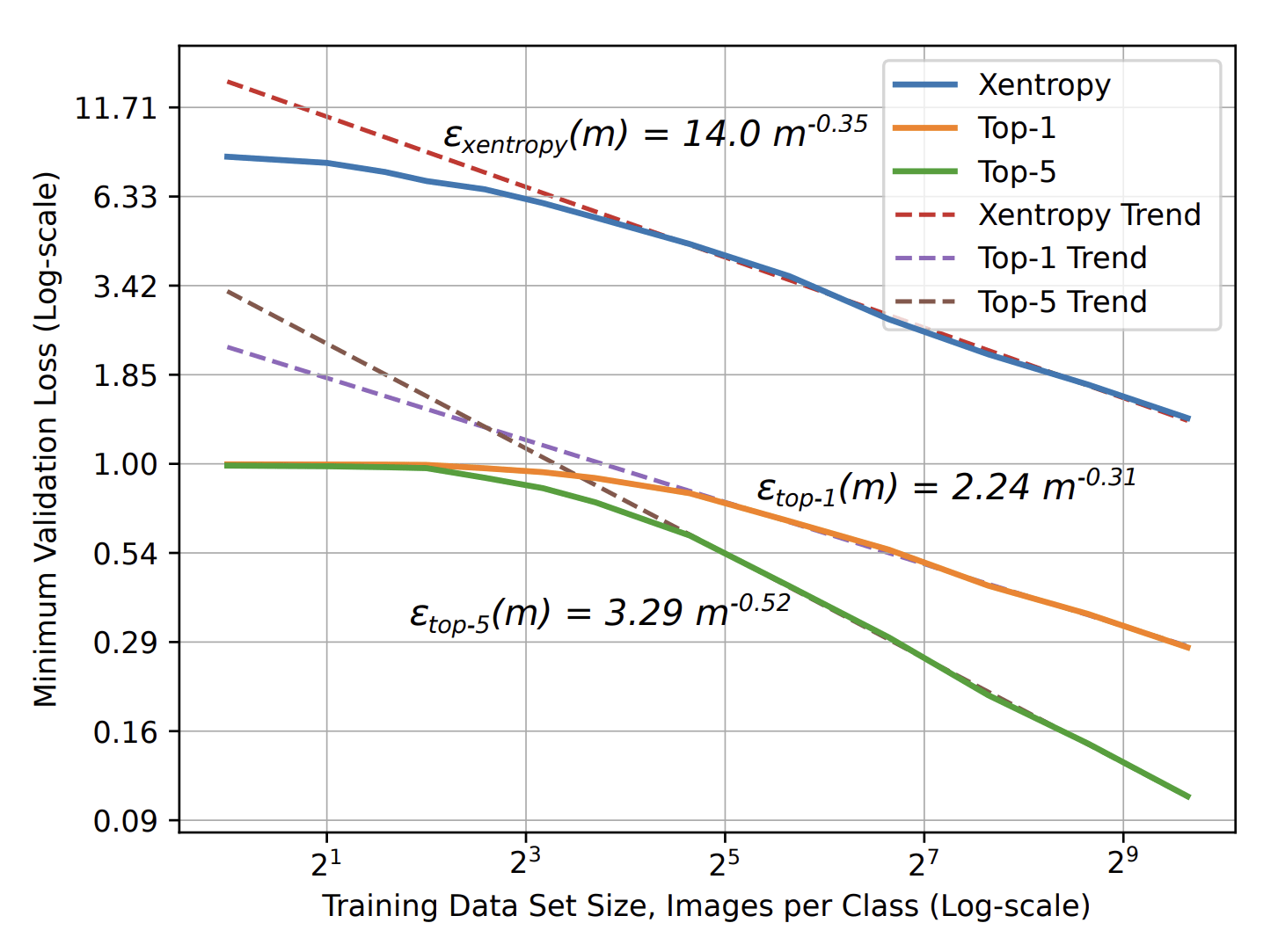
\(\varepsilon\sim P^{-\beta}\)
3/28
Error \(\varepsilon\)
of ML model
Number of training points \(P\)
Measuring diffeomorphisms sensitivity
\(\tau(x)\)
\((x+\eta)\)
\(+\eta\)
\(\tau\)
\(f(\tau(x))\)
\(f(x+\eta)\)
\(x\)
Our model captures the fact that while sensitivity to diffeo decreases, the sensitivity to noise increases
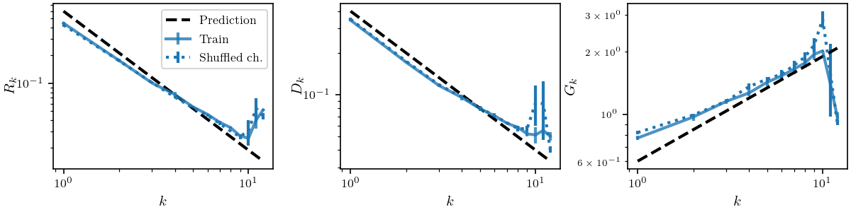
Inverse trend
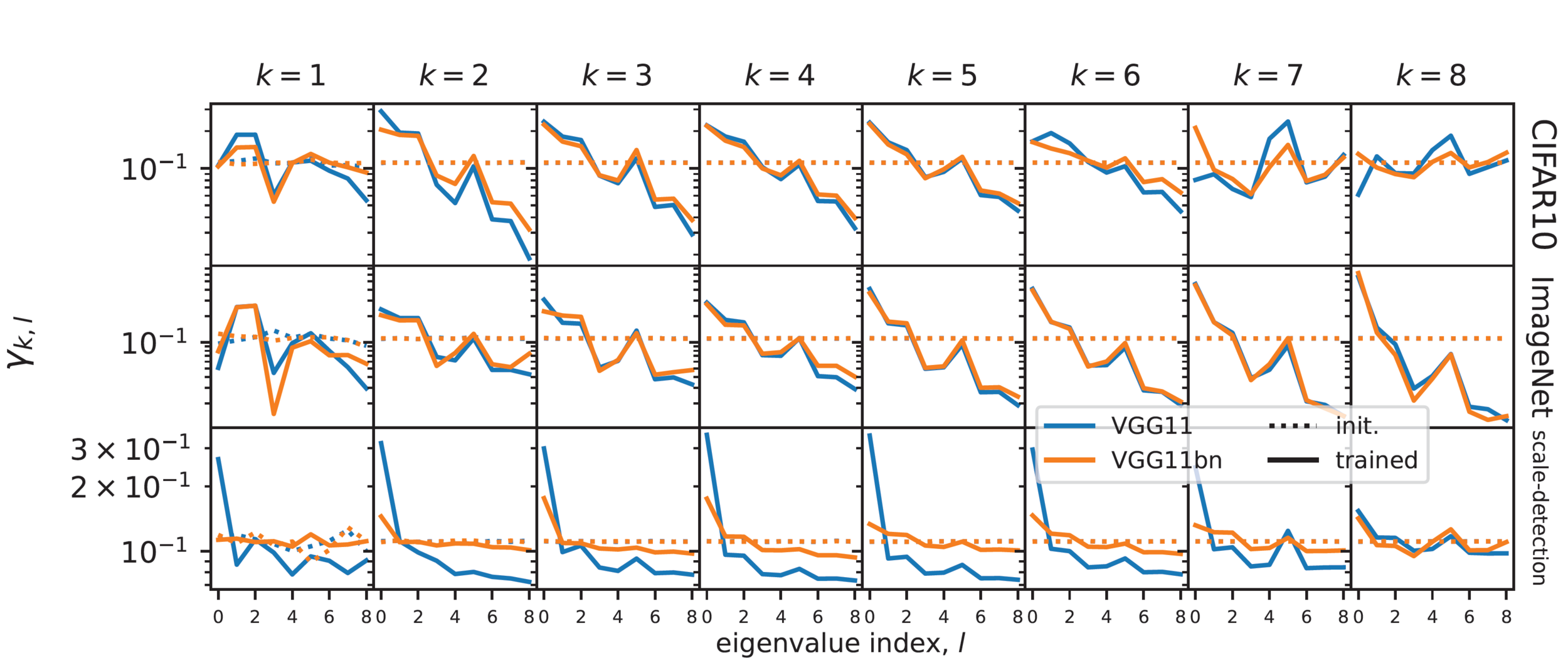
\(\gamma_{k,l}=\mathbb{E}_{c,c'}[\omega^k_{c,c'}\cdot\Psi_l]\)
- \(\omega^k_{c,c'}\): filter at layer \(k\) connecting channel \(c\) of layer \(k\) with channel \(c'\) of layer \(k-1\)
- \(\Psi_l\) : 'Fourier' base for filters, smaller index \(l\) is for more low-pass filters.
Frequency content of filters
Few layers become low-pass: spatial pooling
- Overall \(G_k\) increases
- Using odd activation functions as tanh nullifies this effect.
Noise
Increase of Sensitivity to Noise
Input
Avg Pooling
Layer 1
Layer 2
Avg Pooling
ReLU
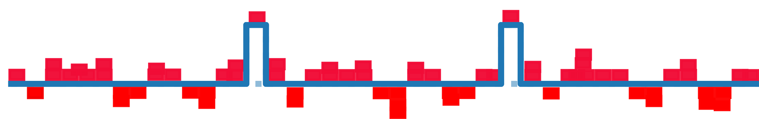
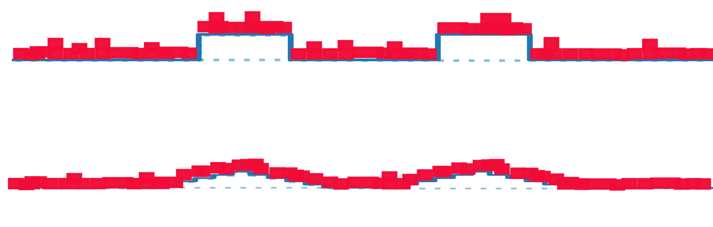
\(G_k = \frac{\mathbb{E}_{x,\eta}\| f_k(x+\eta)-f_k(x)\|^2}{\mathbb{E}_{x_1,x_2}\| f_k(x_1)-f_k(x_2)\|^2}\)
- Difference before and after the noise: noise
- Concentrating average around positive mean
- Constant in depth \(k\)
- Difference of two peaks: one peak
- Squared norm decrease in \(k\)
\(P^*\) points are needed to measure correlations
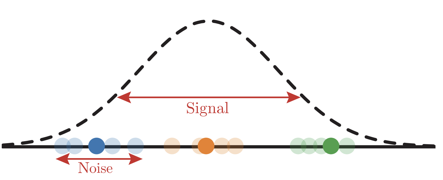
- If \(Prob(label|input\, patch)\) is \(1/n_c\): no correlations
- Signal: ratio std/mean of prob.
- Sampling noise: ratio std/mean of empirical prob
\(\sim[m^L/(mv)]^{-1/2}\)
\(\sim[P/(n_c m v)]^{-1/2}\)
Large \(m,\, n_c,\, P\):
\(P_{corr}\sim n_c m^L\)
One GD step collapses
representations for synonyms
- Data: s-dimensional patches, one-hot encoding out of \(v^s\) possibilities (orthogonalization)
- Network: two-layer fully connected network, second layer Gaussian and frozen, first layer all 1s
- Loss: cross entropy
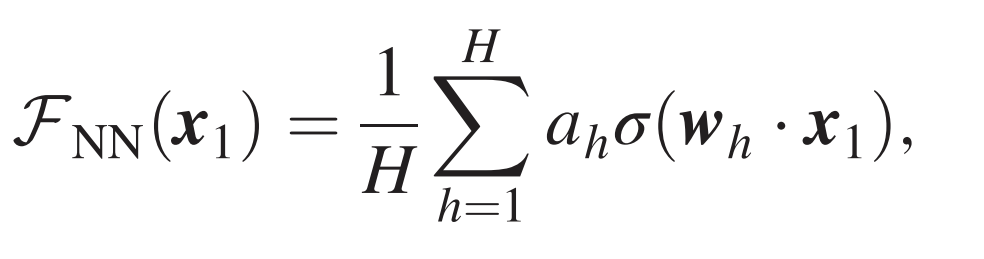
- Network learns the first composition rule of the RHM by building a representation invariant to exchanges of level-1 synonyms.
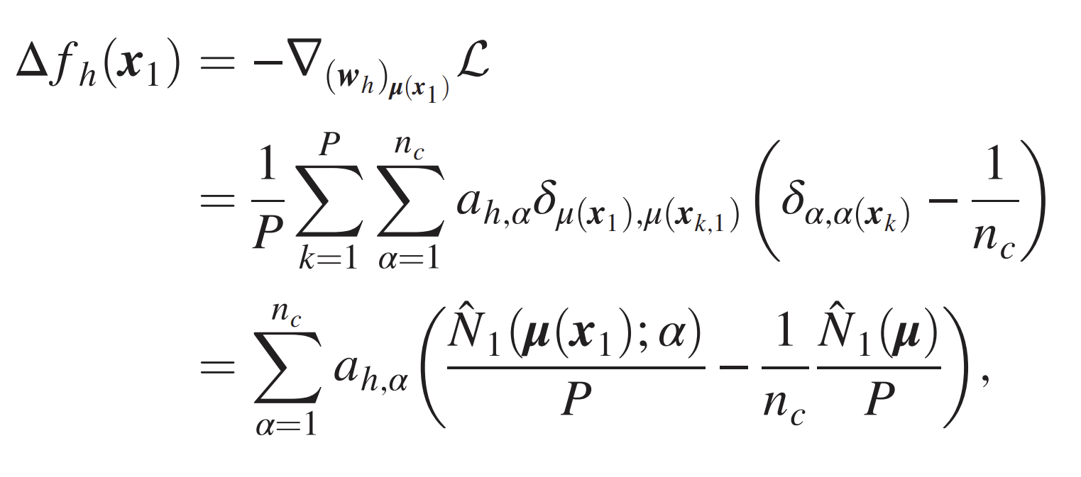
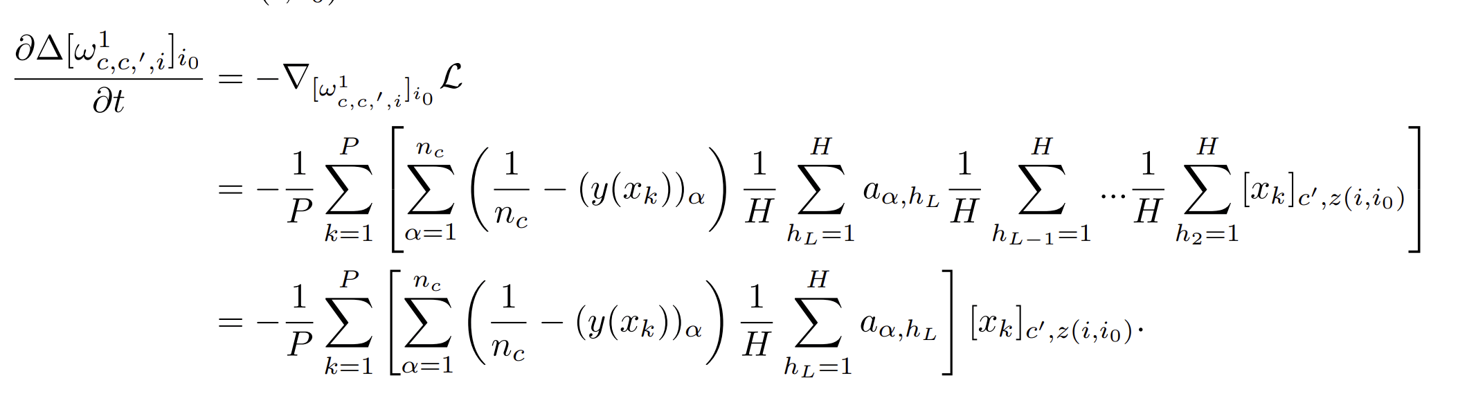
- One GD step: gradients \(\sim\) empirical counting of patches-label
- For \(P>P^*\) they converge to non-empirical, invariant for synonyms

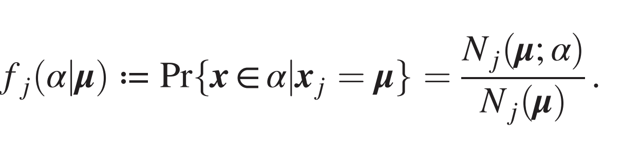
Curse of Dimensionality without correlations
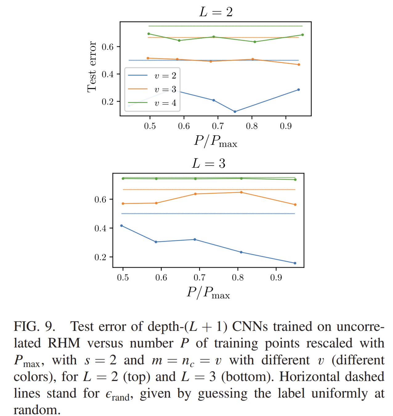
Uncorrelated version of RHM:
- features are uniformly distributed among classes.
- A tuple \(\mu\) in the \(j-\)th patch at level 1 belongs to a class \(\alpha\) with probability \(1/n_c\)
Curse of Dimensionality even for deep nets
Horizontal lines: random error
Which net do we use?
We consider a different version of a Convolutional Neural Network (CNN) without weight sharing
Standard CNN:
- local
- weight sharing
Locally Connected Network (LCN):
- local
weight sharing
One step of GD groups synonyms with \(P^*\) points
- Data: SRHM with \(L\) levels, with one-hot encoding of the \(v\) informative features, empty otherwise
- Network: LCN with \(L\) layers, readout layer Gaussian and frozen
- GD update of one weight at bottom layer depends on just one input position
- On average it is informative with \(p=(s_0+1)^{-L}\)
- Just a fraction of data points \(P'=p \cdot P\) contribute
- For \(P=(1/p) P^*_0\) the GD updates are as sparseless case with \(P^*_0\) points
- At that scale, a single step groups together representations with equal correlation with label
Single input feature!
The learning algorithm
- Regression of a target function \(f^*\) from \(P\) examples \(\{x_i,f^*(x_i)\}_{i=1,...,P}\).
- Interest in kernels renewed by lazy neural networks
f_P(x)=\sum_{i=1}^P a_i K(x_i,x)
\text{min}\left[\sum\limits_{i=1}^P\left|f^*(x_i)-f_P(x_i)\right|^2 +\lambda ||f_P||_K^2\right]
Train loss:
\(K(x,y)=e^{-\frac{|x-y|}{\sigma}}\)
E.g. Laplacian Kernel
- Kernel Ridge Regression (KRR):
Fixed Features
Failure and success of Spectral Bias prediction..., [ICML22]
- Key object: generalization error \(\varepsilon_t\)
- Typically \(\varepsilon_t\sim P^{-\beta}\), \(P\) number of training data
Predicting generalization of KRR
[Canatar et al., Nature (2021)]
General framework for KRR
- Predicts that KRR has a spectral bias in its learning:
\(\rightarrow\) KRR learns the first \(P\) eigenmodes of \(K\)
\(\rightarrow\) \(f_P\) is self-averaging with respect to sampling
- Obtained by replica theory
- Works well on some real data for \(\lambda>0\)
\(\rightarrow\) what is the validity limit?
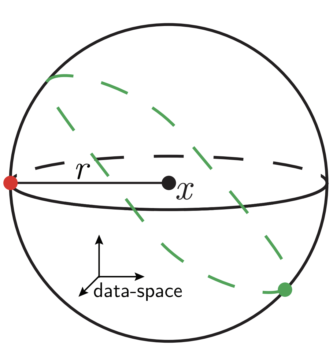
Our toy model
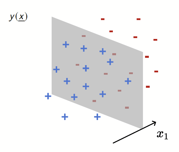
Depletion of points around the interface
p(x_1)= \frac{1}{\mathcal{Z}}\color{red}{|x_1|^\chi}\color{black} e^{-x_1^2}
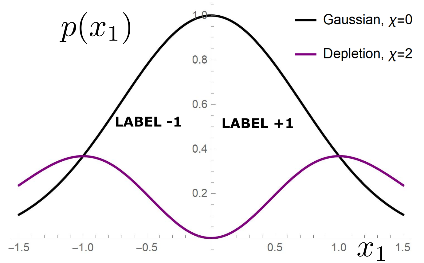
Data: \(x\in\mathbb{R}^d\)
Label: \(f^*(x_1,x_{\bot})=\text{sign}[x_1]\)
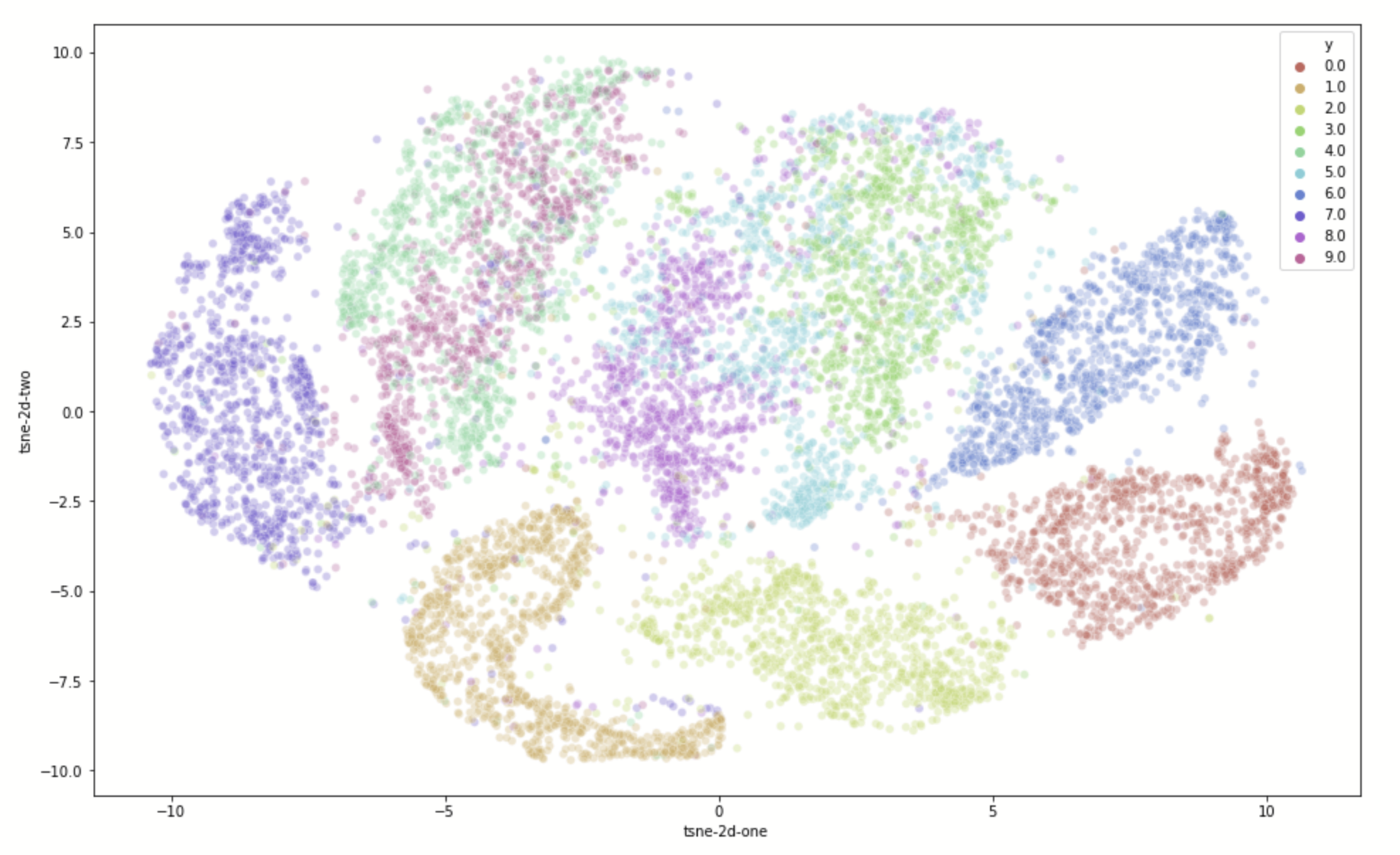
Motivation:
evidence for gaps between clusters in datasets like MNIST
Predictor in the toy model
(1) Spectral bias predicts a self-averaging predictor controlled by a characteristic length \( \ell(\lambda,P) \propto \lambda/P \)
For fixed regularizer \(\lambda/P\):
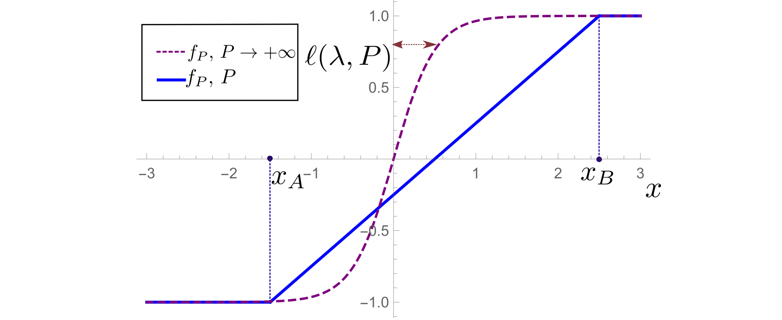
(2) When the number of sampling points \(P\) is not enough to probe \( \ell(\lambda,P) \):
- \(f_P\) is controlled by the statistics of the extremal points \(x_{\{A,B\}}\)
- spectral bias breaks down.
\(d=1\)
\varepsilon_B \sim P^{-(1+\frac{1}{d})\frac{1+\chi}{1+d+\chi}}
\varepsilon_t \sim P^{-\frac{1+\chi}{d+\chi}}
\neq
Different predictions for
\(\lambda\rightarrow0^+\)
- For \(\chi=0\): equal
- For \(\chi>0\): equal for \(d\rightarrow\infty\)
\lambda^*_{d,\chi}\sim P^{-\frac{1}{d+\chi}}
Crossover at:
\(\lambda\)
Spectral bias failure
Spectral bias success
Takeaways and Future directions
For which kind of data spectral bias fails?
Depletion of points close to decision boundary
Still missing a comprehensive theory for
KRR test error for vanishing regularization
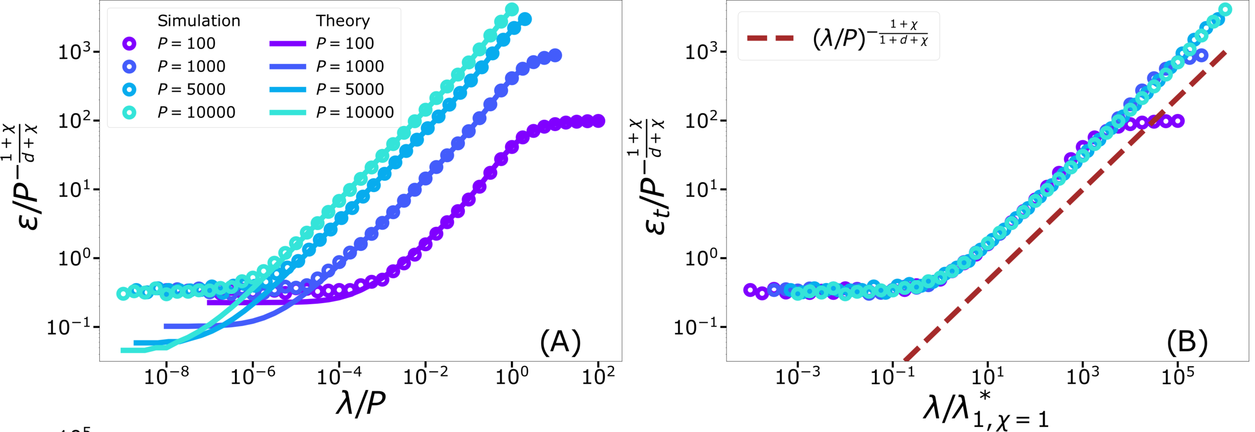
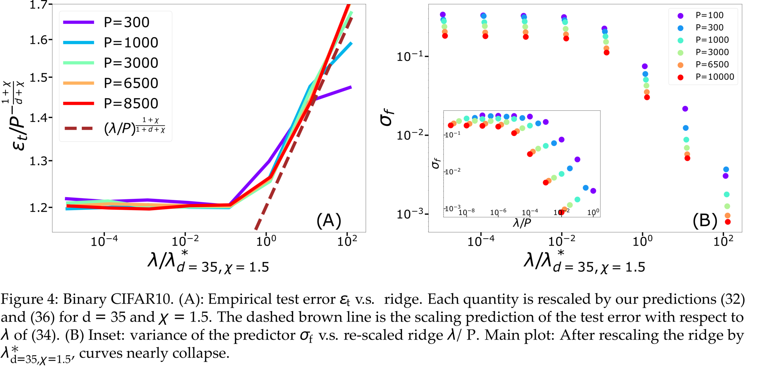
Test error: 2 regimes
For fixed regularizer \(\lambda/P\):
\(\rightarrow\) Predictor controlled by extreme value statistics of \(x_B\)
\(\rightarrow\) Not self-averaging: no replica theory
(2) For small \(P\): predictor controlled by extremal sampled points:
\(x_B\sim P^{-\frac{1}{\chi+d}}\)
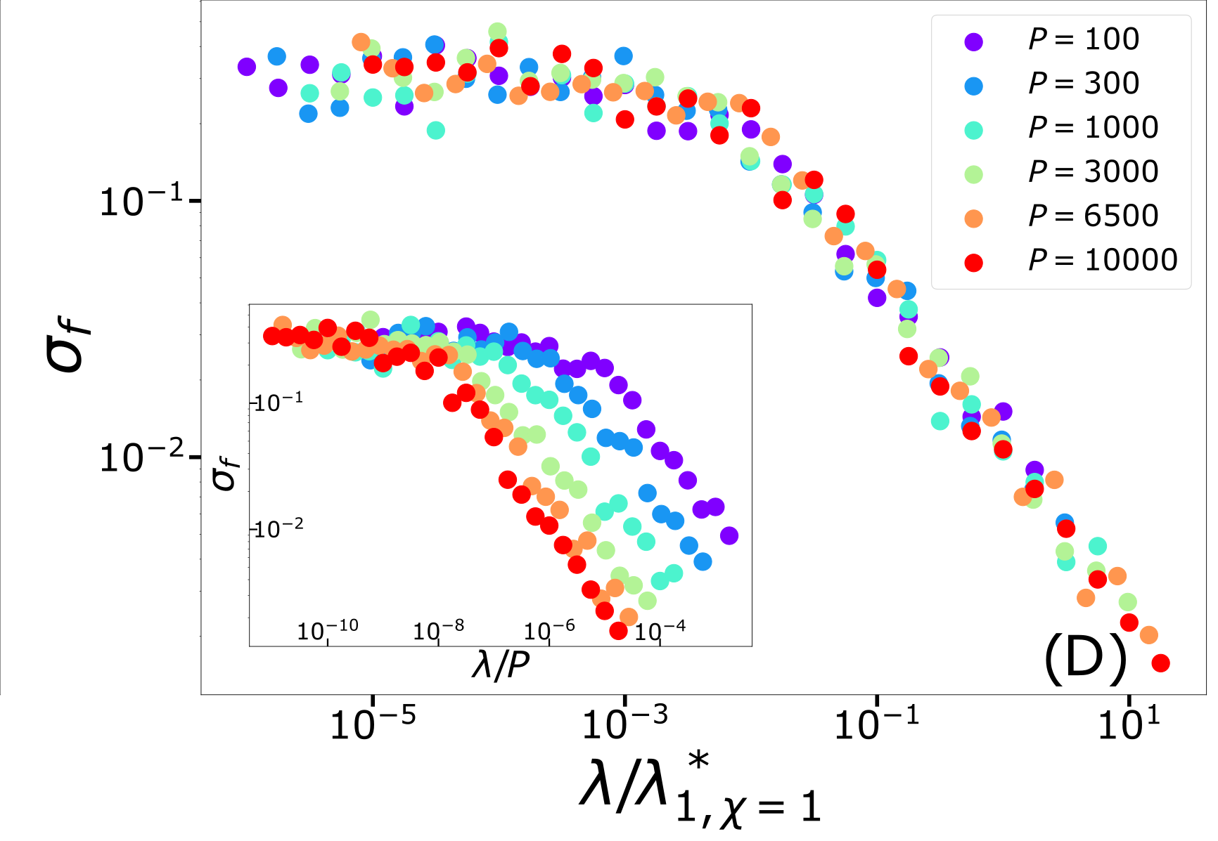
The self-averageness crossover
\(\rightarrow\) Comparing the two characteristic lengths \(\ell(\lambda,P)\) and \(x_B\):
\lambda^*_{d,\chi}\sim P^{-\frac{1}{d+\chi}}
\sigma_f = \langle [f_{P,1}(x_i) - f_{P,2}(x_i)]^2 \rangle
\varepsilon_B \sim P^{-(1+\frac{1}{d})\frac{1+\chi}{1+d+\chi}}
\varepsilon_t \sim P^{-\frac{1+\chi}{d+\chi}}
\neq
Different predictions for
\(\lambda\rightarrow0^+\)
- For \(\chi=0\): equal
- For \(\chi>0\): equal for \(d\rightarrow\infty\)
- Replica predictions works even for small \(d\), for large ridge.
- For small ridge: spectral bias prediction, if \(\chi>0\) correct just for \(d\rightarrow\infty\).
- To test spectral bias, we solved eigendecomposition of Laplacian kernel for non-uniform data, using quantum mechanics techniques (WKB).
- Spectral bias prediction based on Gaussian approximation: here we are out of Gaussian universality class.
Technical remarks:
Fitting CIFAR10
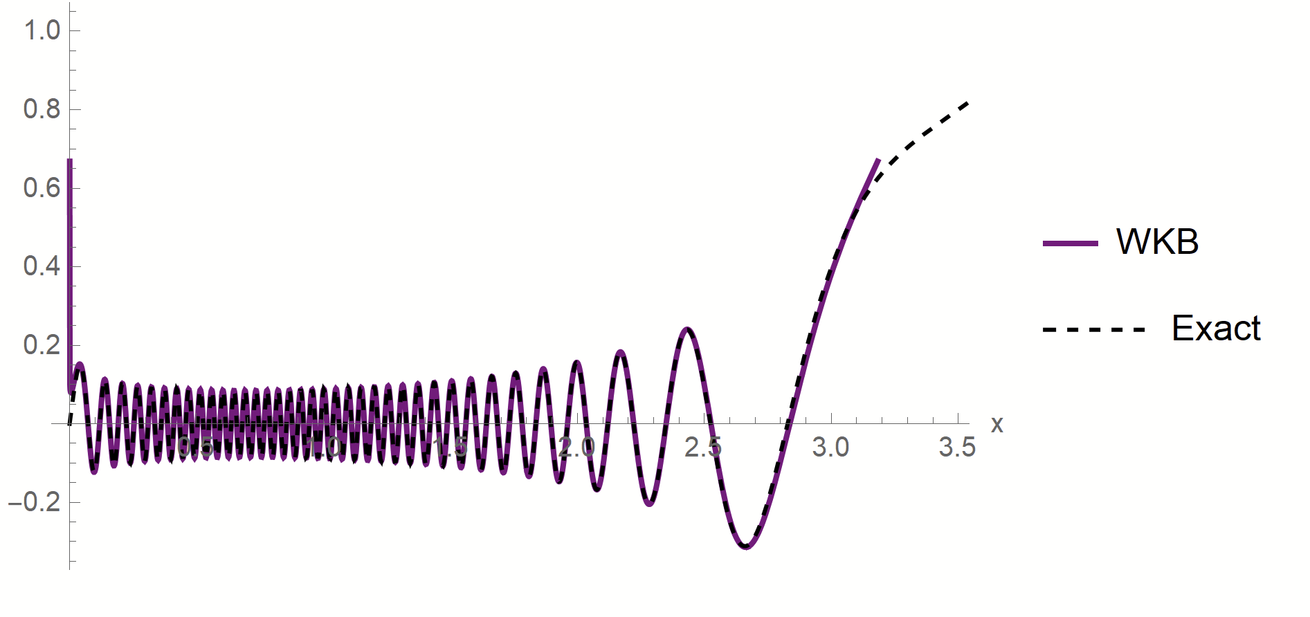
Proof:
- WKB approximation of \(\phi_\rho\) in [\(x_1^*,\,x_2^*\)]:
\(\phi_\rho(x)\sim \frac{1}{p(x)^{1/4}}\left[\alpha\sin\left(\frac{1}{\sqrt{\lambda_\rho}}\int^{x}p^{1/2}(z)dx\right)+\beta \cos\left(\frac{1}{\sqrt{\lambda_\rho}}\int^{x}p^{1/2}(z)dx\right)\right]\)
x_1^*
x_2^*
- MAF approximation outside [\(x_1^*,\,x_2^*\)]
\(x_1*\sim \lambda_\rho^{\frac{1}{\chi+2}}\)
\(x_2*\sim (-\log\lambda_\rho)^{1/2}\)
- WKB contribution to \(c_\rho\) is dominant in \(\lambda_\rho\)
- Main source WKB contribution:
first oscillations
Formal proof:
- Take training points \(x_1<...<x_P\)
- Find the predictor in \([x_i,x_{i+1}]\)
- Estimate contribute \(\varepsilon_i\) to \(\varepsilon_t\)
- Sum all the \(\varepsilon_i\)
Characteristic scale of predictor \(f_P\), \(d=1\)
\sigma^2 \partial_x^2 f_P(x) =\left(\frac{\sigma}{\lambda/P}p(x)+1\right)f_P(x)-\frac{\sigma}{\lambda/P}p(x)f^*(x)
Minimizing the train loss for \(P \rightarrow \infty\):
\(\rightarrow\) A non-homogeneous Schroedinger-like differential equation
\(\rightarrow\) Its solution yields:
\ell(\lambda,P)\sim \left(\frac{\lambda\sigma}{P}\right)^{\frac{1}{(2+\chi)}}
Characteristic scale of predictor \(f_P\), \(d>1\)
- Let's consider the predictor \(f_P\) minimizing the train loss for \(P \rightarrow \infty\).
f_P(x)=\int d^d\eta \frac{p(\eta) f^*(\eta)}{\lambda/P} G(x,\eta)
- With the Green function \(G\) satisfying:
\int d^dy K^{-1}(x-y) G_{\eta}(y) = \frac{p(x)}{\lambda/P} G_{\eta}(x) + \delta(x-\eta)
- In Fourier space:
\mathcal{F}[K](q)^{-1} \mathcal{F}[G_{\eta}](q) = \frac{1}{\lambda/P} \mathcal{F}[p\ G_{\eta}](q) + e^{-i q \eta}
- In Fourier space:
\mathcal{F}[K](q)^{-1} \mathcal{F}[G_{\eta}](q) = \frac{1}{\lambda/P} \mathcal{F}[p\ G_{\eta}](q) + e^{-i q \eta}
\begin{aligned}
\mathcal{F}[G](q)&\sim q^{-1-d}\ \ \ \text{for}\ \ \ q\gg q_c\\
\mathcal{F}[G](q)&\sim \frac{\lambda}{P}q^\chi\ \ \ \text{for}\ \ \ q\ll q_c\\
\text{with}\ \ \ q_C&\sim \left(\frac{\lambda}{P}\right)^{-\frac{1}{1+d+\chi}}
\end{aligned}
- Two regimes:
- \(G_\eta(x)\) has a scale:
\ell(\lambda,P)\sim 1/q_c\sim \left(\frac{\lambda}{P}\right)^{\frac{1}{1+d+\chi}}
PhD_defense_public
By umberto_tomasini


