How Data Structures affect Generalization in Kernel Methods and Deep Learning

Umberto Maria Tomasini
1/28
Failure and success of the spectral bias prediction for Laplace Kernel Ridge Regression: the case of low-dimensional data
UMT, Sclocchi, Wyart
ICML 22
How deep convolutional neural network
lose spatial information with training
UMT, Petrini, Cagnetta, Wyart
ICLR23 Workshop,
Machine Learning: Science and Technology 2023
How deep neural networks learn compositional data:
The random hierarchy model
Cagnetta, Petrini, UMT, Favero, Wyart
PRX 24
How Deep Networks Learn Sparse and Hierarchical Data:
the Sparse Random Hierarchy Model
UMT, Wyart
ICML 24
Clusterized data
Invariance to deformations
Invariance to deformations
Hierarchy
Hierarchy
2/28
The puzzling success of Machine Learning
- Machine learning is highly effective across various tasks
- Scaling laws: More training data leads to better performance
Curse of dimensionality occurs when learning structureless data in high dimension \(d\):
- Slow decay: \(\beta=1/d\)
- Number of training data to learn is exponential in \(d\).
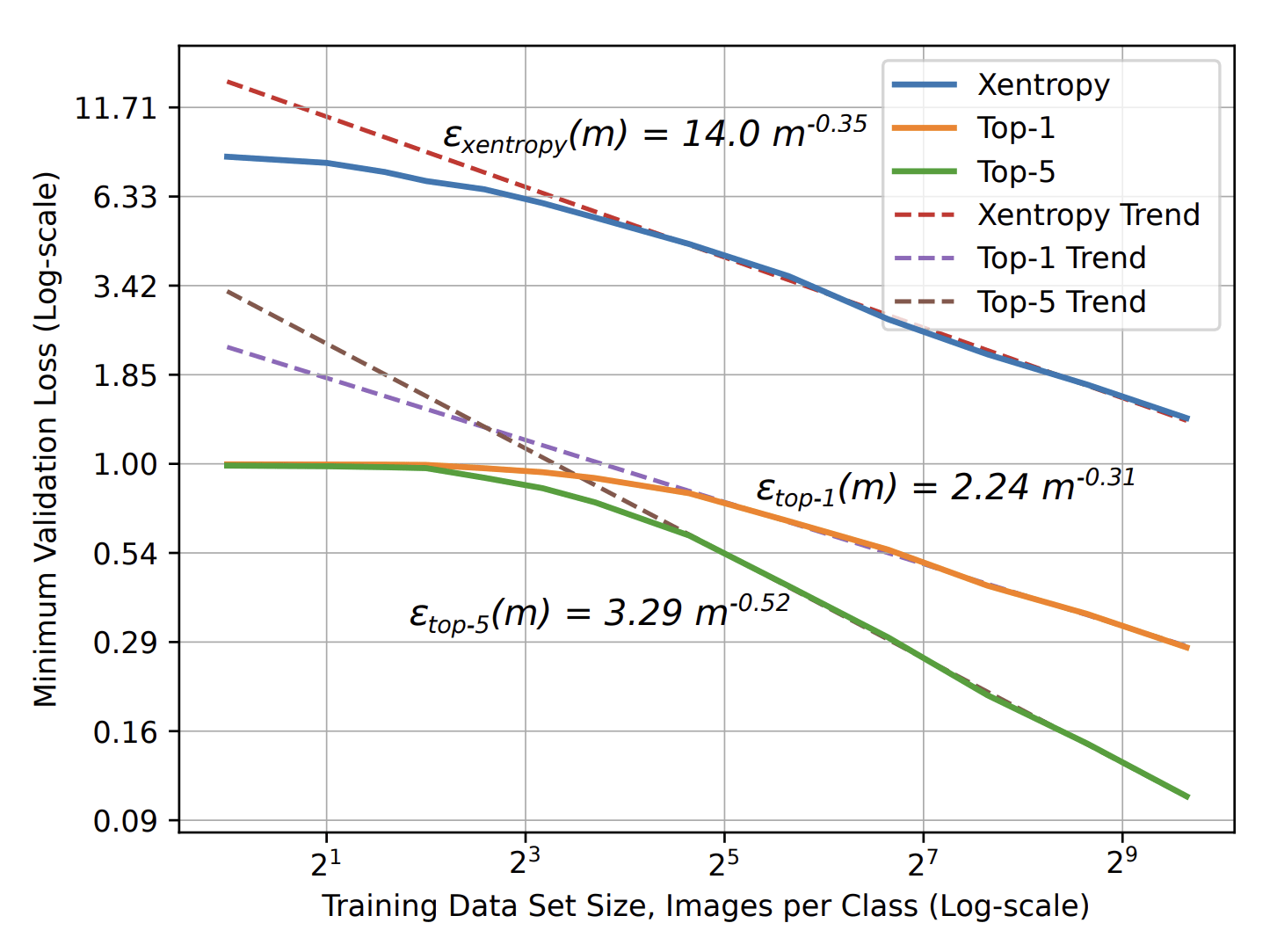
- Image Classification: \(\beta=\,0.3\,-\,0.5\)
- Speech Recognition: \(\beta\approx\,0.3\)
- Language Modeling: \(\beta\approx\,0.1\)
VS
\(\varepsilon\sim P^{-\beta}\)
3/28
\(\Rightarrow\) Data must be structured and
Machine Learning should capture such structure.
Key questions motivating this thesis:
- What constitutes a learnable structure?
- How does Machine Learning exploit it?
- How many training points are required?
4/28
Data must be Structured
Data properties learnable by simple methods
- Data lies on a smooth low-dimensional manifold,
- Smoothness,
\(\Rightarrow\) Kernel Methods
3. Task depend on a few coordinates,
e.g. \(f(x)=f(x_1)\),
\(\Rightarrow\) Shallow Networks
[Bennet 69, Pope 21, Goldt 20, Smola 98, Rosasco 17, Caponetto and De Vito 05-07, Steinwart 09, Steinwart 20, Loureiro 21, Cui 21, Richards 21, Xu 21, Patil 21, Kanagawa 18, Jin 21, Bordelon 20, Canatar 21, Spigler 20, Jacot 20, Mei 21, Bahri 24]
[UMT, Sclocchi, Wyart, ICML 22]
Properties 1-3 not enough:
- Kernels and shallow nets underperform compared to deep nets on real data
Why? What structure do they learn?
[Barron 93, Bach 17, Bach 20, Schmidt-Hieber 20,
Yehudai and Shamir 19, Ghorbani 19-20, Wei 19, Paccolat 20, Dandi 23]
5/28
Reducing complexity with depth
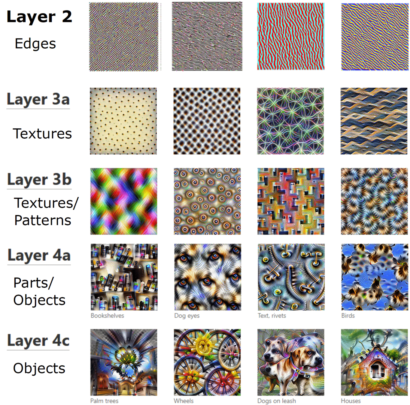
Deep networks build increasingly abstract representations with depth (also in brain)
- How many training points are needed?
- Why are these representations effective?
Intuition: reduces complexity of the task, ultimately beating curse of dimensionality.
- Which irrelevant information is lost ?
Two ways for losing information
by learning invariances
Discrete
Continuous
[Zeiler and Fergus 14, Yosinski 15, Olah 17, Doimo 20,
Van Essen 83, Grill-Spector 04]
[Shwartz-Ziv and Tishby 17, Ansuini 19, Recanatesi 19, ]
[Bruna and Mallat 13, Mallat 16, Petrini 21]
6/28
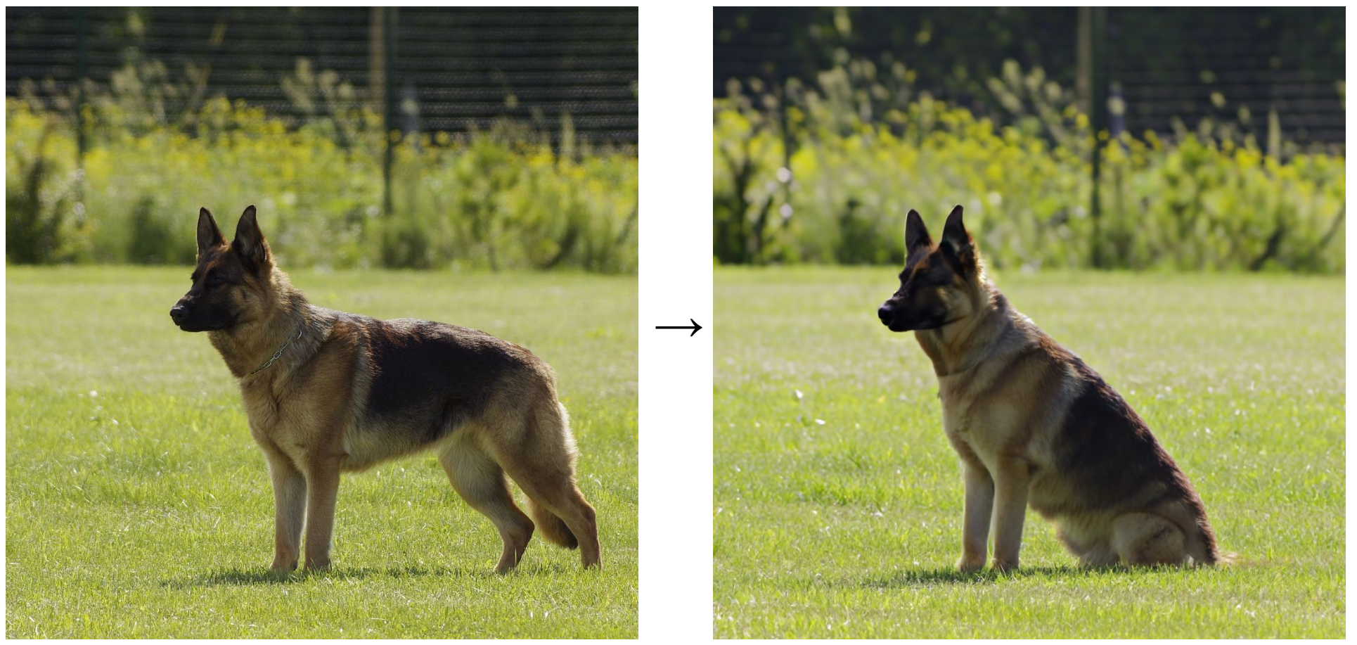
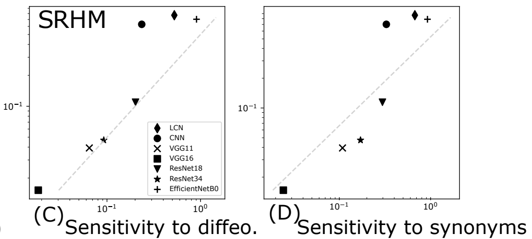
How learning continuous invariances
correlates with performance
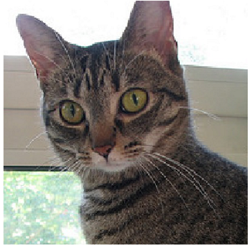
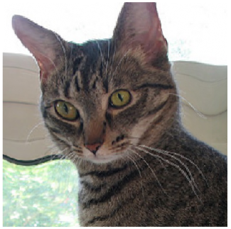
Test error correlates with sensitivity to diffeo
Test error anti-correlates with sensitivity to noise
\((x+\eta)\)
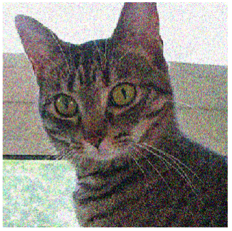
\(x\)
Can we explain this phenomenology?
[Petrini21]
\(x\)
\(\tau(x)\)
Sensitivity to diffeo
Test error
+Sensitive
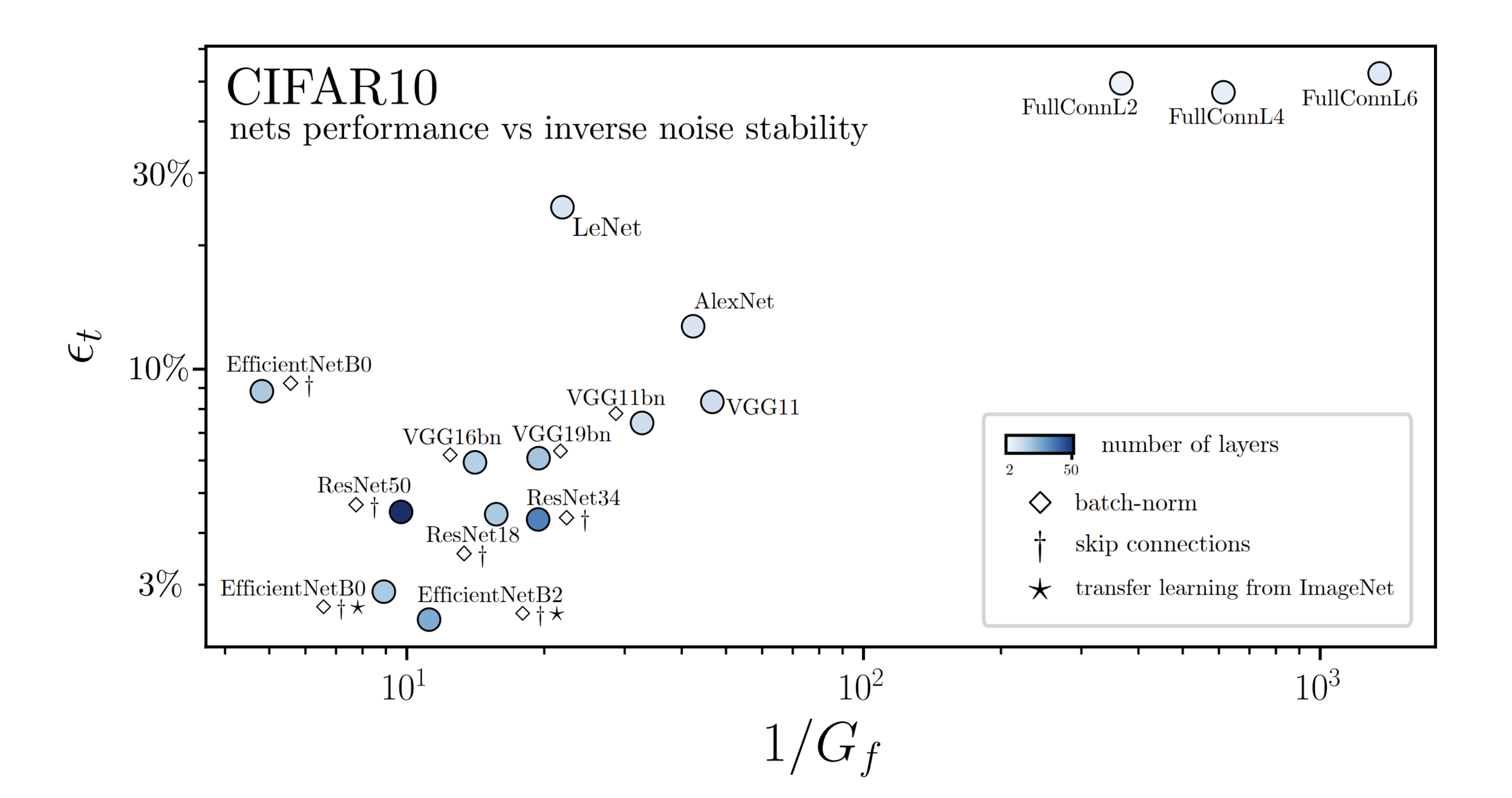
Inverse of Sensitivity to noise
Test error
+Sensitive
7/28
- Compositional structure of data,
- Hierarchical structure of data,
This thesis:
data properties learnable by deep networks
[Poggio 17, Mossel 16, Malach 18-20, Schmdit-Hieber 20, Allen-Zhu and Li 24]
3. Data are sparse,
4. The task is stable to transformations.
[Bruna and Mallat 13, Mallat 16, Petrini 21]
How many training points are needed for deep networks?
8/28
Outline
Part I: analyze mechanistically why the best networks are the most sensitive to noise.
Part II: introduce a hierarchical model of data to quantify the gain in number of training points.
Part III: understand why the best networks are the least sensitive to diffeo, in an extension of the hierarchical model.
9/28
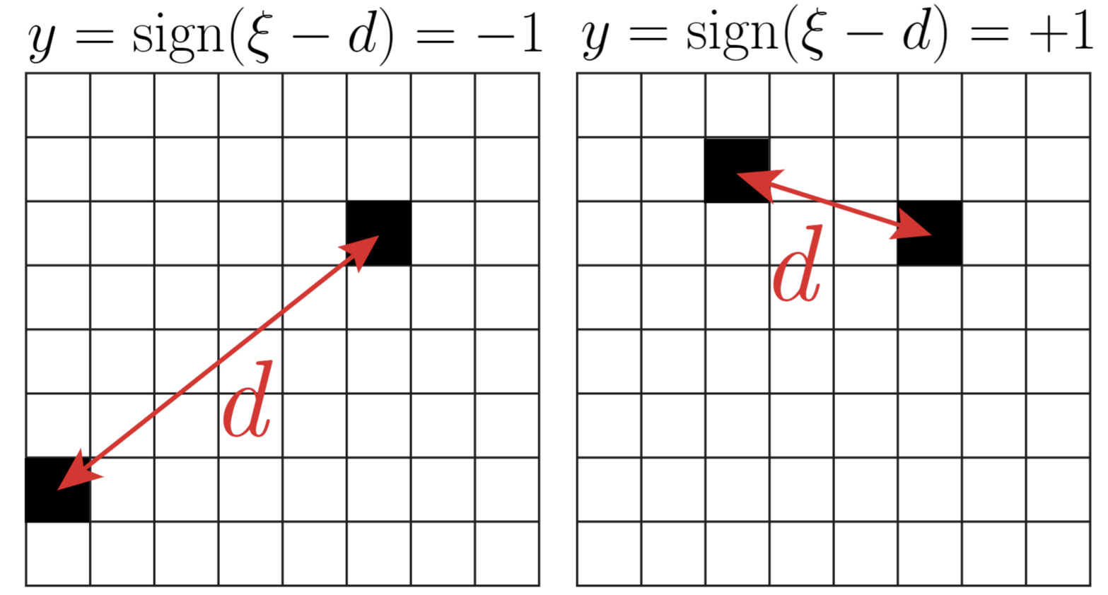
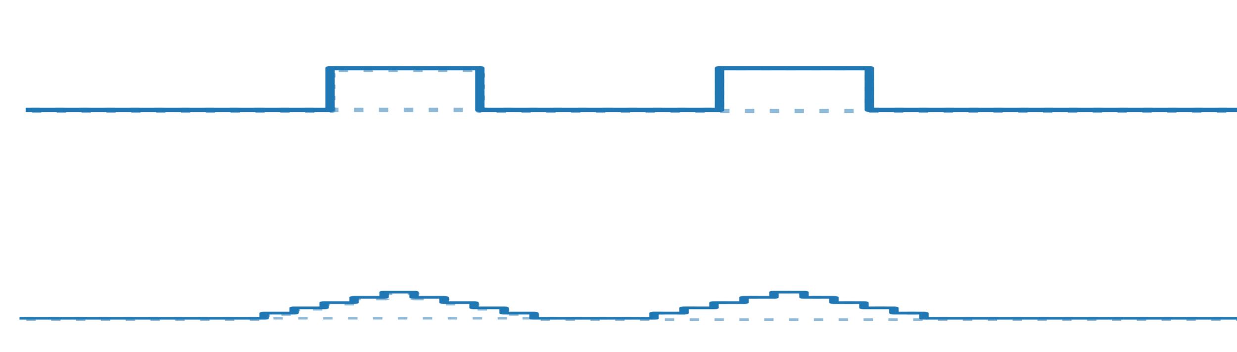
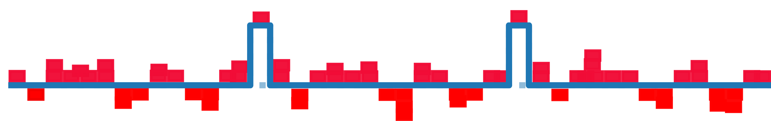
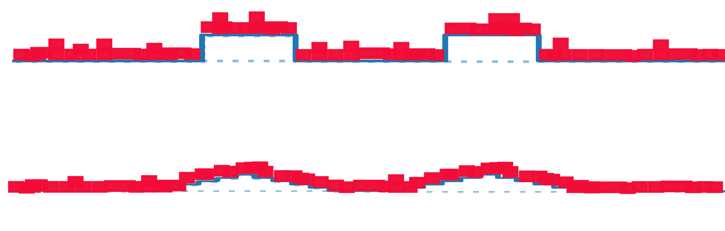
Part I: A simple task captures the inverse trend
\(d<\xi\,\rightarrow\, y=1\)
\(d>\xi\,\rightarrow\, y=-1\)
\(d\): distance between active pixels
\(\xi\): characteristic scale
[UMT, Petrini, Cagnetta, Wyart, ICLR23 Workshop,
Machine Learning: Science and Technology 2023]
- Position of the features is not relevant.
- Networks must become insensitive to diffeo.
- Deep networks learn solutions using average pooling up to scale \(\xi\)
- They become sensitive to noise and insensitive to diffeo
\(y=1\)
\(y=-1\)
\(\xi\)
\(\xi\)
10/28
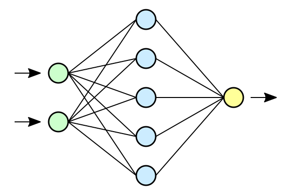
How Avg Pooling affects deep representations
- Analyzing one active pixel at the time
- Network: stack of ReLU convolutional layers with homogeneous filters
- Representations wider and smaller with depth
- Diffeomorphism: less impact with depth since representations are wider

Input
Avg Pooling
Layer 1
Layer 2
Avg Pooling
- Size of noise remains constant for layer >1 while size of representation decreases
- Sensitivity to noise increases!
ReLU
Concentrates around
positive mean!
Noise
11/28
Takeaways
- To become insensitive to diffeo, deep networks build average pooling solutions
- A mechanistic consequence: Average pooling piles up positive noise, increasing the sensitivity to noise
- Using odd activations functions as \(tanh\) reduces sensitivity to noise
- We saw how to lose information about the exact position of the features by learning to be insensitive to diffeo.
- Still no notion about how to compose these features to build the meaning of the image
Next:
12/28
Part II: Hierarchical structure
Do deep hierarchical representations exploit the hierarchical structure of data?
[Poggio 17, Mossel 16, Malach 18-20, Schmdit-Hieber 20, Allen-Zhu and Li 24]
How many training points?
Quantitative predictions in a model of data
[Cagnetta, Petrini, UMT, Favero, Wyart, PRX 24]
sofa
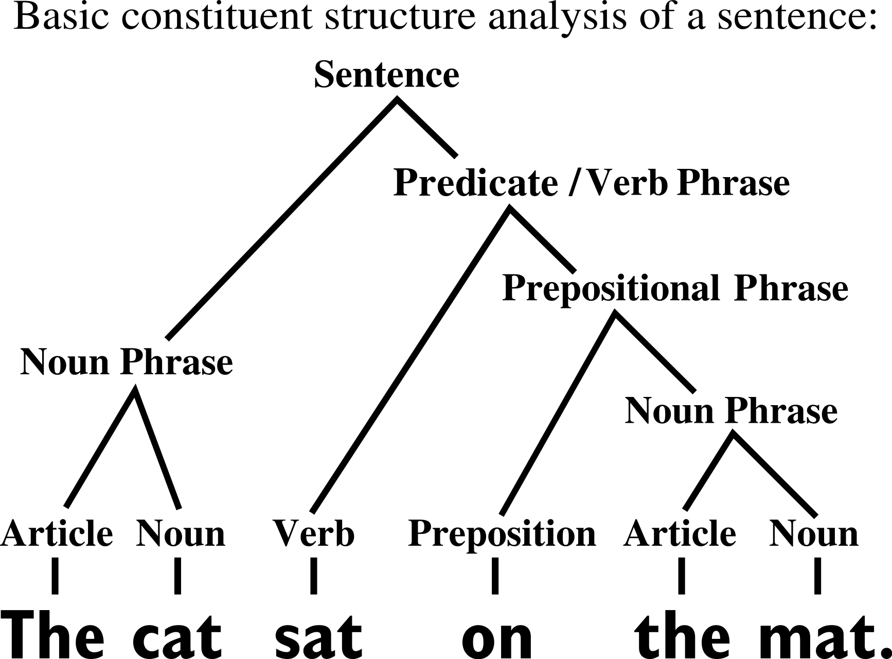
[Chomsky 1965]
[Grenander 1996]
13/28
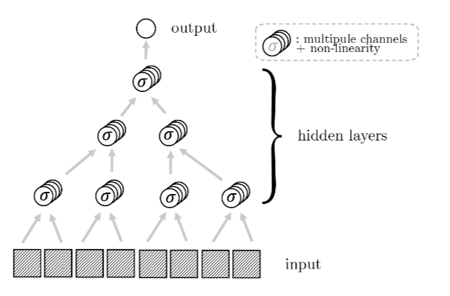
Random Hierarchy Model
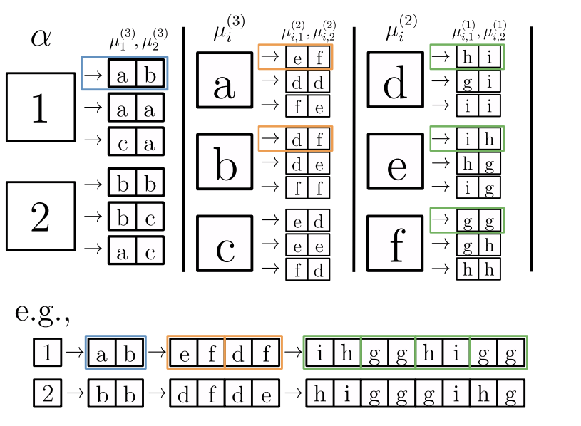
- Generative model: label generates a patch of \(s\) features, chosen from vocabulary of size \(v\)
- Patches chosen randomly from \(m\) different random choices, called synonyms
- Each label is represented by different patches (no overlap)
- Generation iterated \(L\) times with a fixed tree topology.
- Dimension input image: \(d=s^L\)
- Number of data: exponential in \(d\), memorization not practical.
14/28
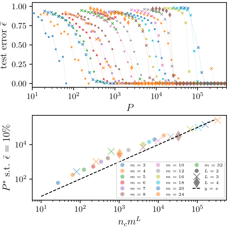
Deep networks beat the curse of dimensionality
\(P^*\)
\(P^*\sim n_c m^L\)
- Polynomial in the input dimension \(s^L\)
- Beating the curse
- Shallow network \(\rightarrow\) cursed by dimensionality
- Depth is key to beat the curse
15/28
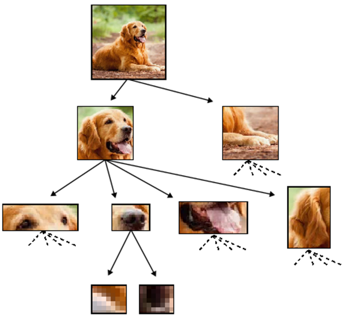
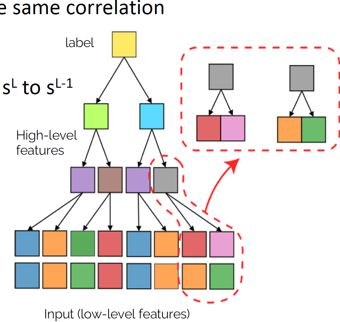
How deep networks learn the hierarchy?
- Intuition: build a hierarchical representation mirroring the hierarchical structure. How to build such representation?
- Start from the bottom. Group synonyms: learn that patches in input correspond to the same higher-level feature
- Collapse representations for synonyms, lowering dimension from \(s^L\) to \(s^{L-1}\)
- Iterate \(L\) times to get hierarchy
How many training points are needed to group synonyms?
16/28
Grouping synonyms by correlations
- Synonyms are patches with same correlation with the label
- Measure correlations by counting
- Large enough training set is required to overcome sampling noise:
- \(P^*\sim n_c m^L\), same as sample complexity
- Simple argument: for \(P>P^*\) one step of Gradient Descent uses the synonyms-label correlations to collapse representations of synonyms
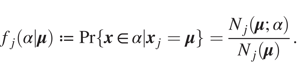
Patch \(\mu\)
Label \(\alpha\)
17/28
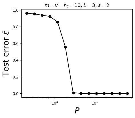
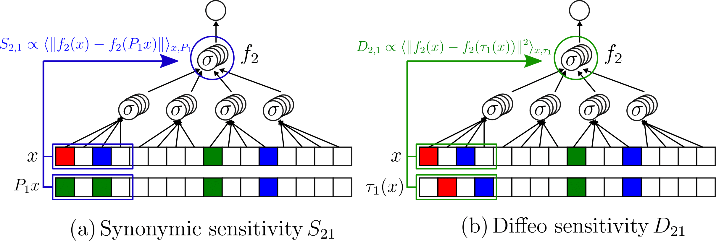
Testing whether deep representations collapse for synonyms
At \(P^*\) the task and the synonyms are learnt
- How much changing synonyms at first level in data change second layer representation (sensitivity)
- For \(P>P^*\) drops
1.0
0.5
0.0
\(10^4\)
Training set size \(P\)
18/28
Takeaways
- Deep networks learn hierarchical tasks with a number of data polynomial in the input dimension
- They do so by developing internal representations invariant to synonyms exchange
Limitations
- To think about images, missing invariance to smooth transformations
- RHM is brittle: a spatial transformation changes the structure/label
Part III
- Extension of RHM to connect with images
- Useful to understand why good networks develop representations insensitive to diffeomorphisms
19/28
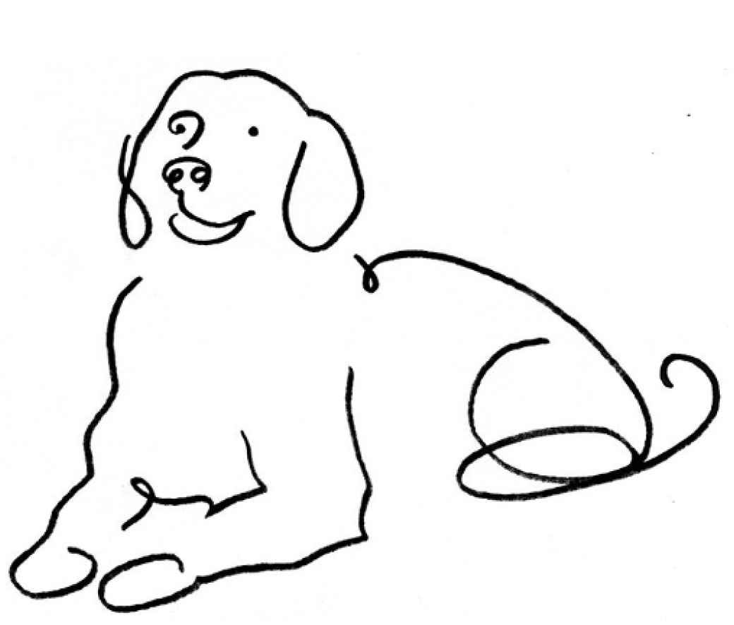
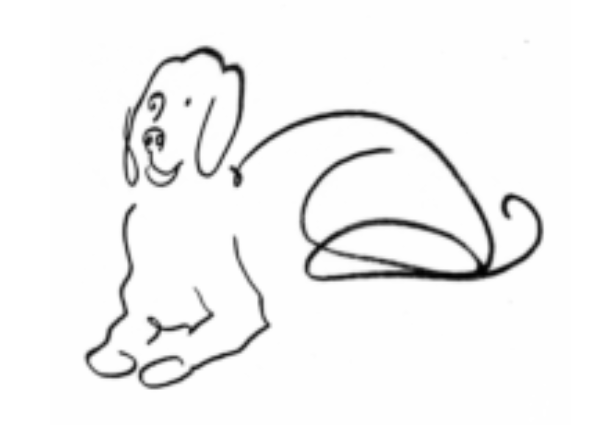
Key insight: sparsity brings invariance to diffeo
- Humans can classify images even from sketches
- Why? Images are made by local and sparse features.
- Their exact positions do not matter.
- \(\rightarrow\) invariance of the task to small local transformations, like diffeomorphisms.
- We incorporate this simple idea in a model of data
[Tomasini, Wyart, ICML 24]
20/28
Sparse Random Hierarchy Model
- Keeping the hierarchical structure
- Each feature is embedded in a sub-patch with \(s_0\) uninformative features.
- The uninformative features are in random positions.
- They generate just uninformative features
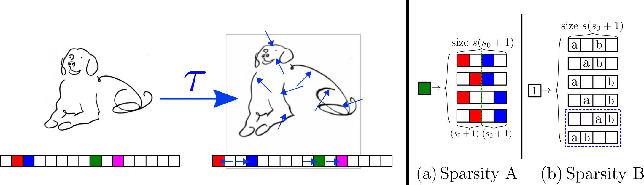
Sparsity\(\rightarrow\) Invariance to feature displacements (diffeo)
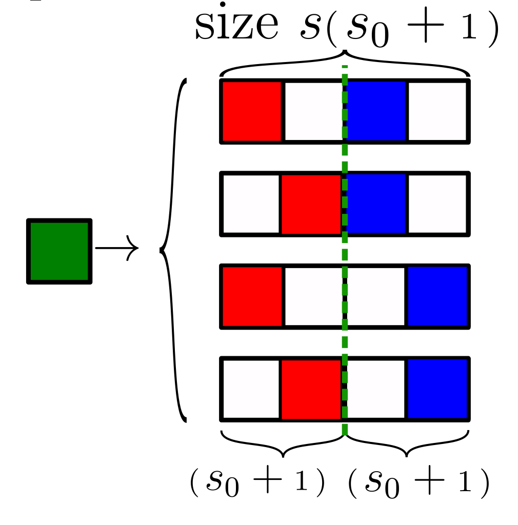
- Very sparse data, \(d=s^L(s_0+1)^L\)

Sparsity \(\rightarrow\) invariance to features displacements (diffeo)

21/28
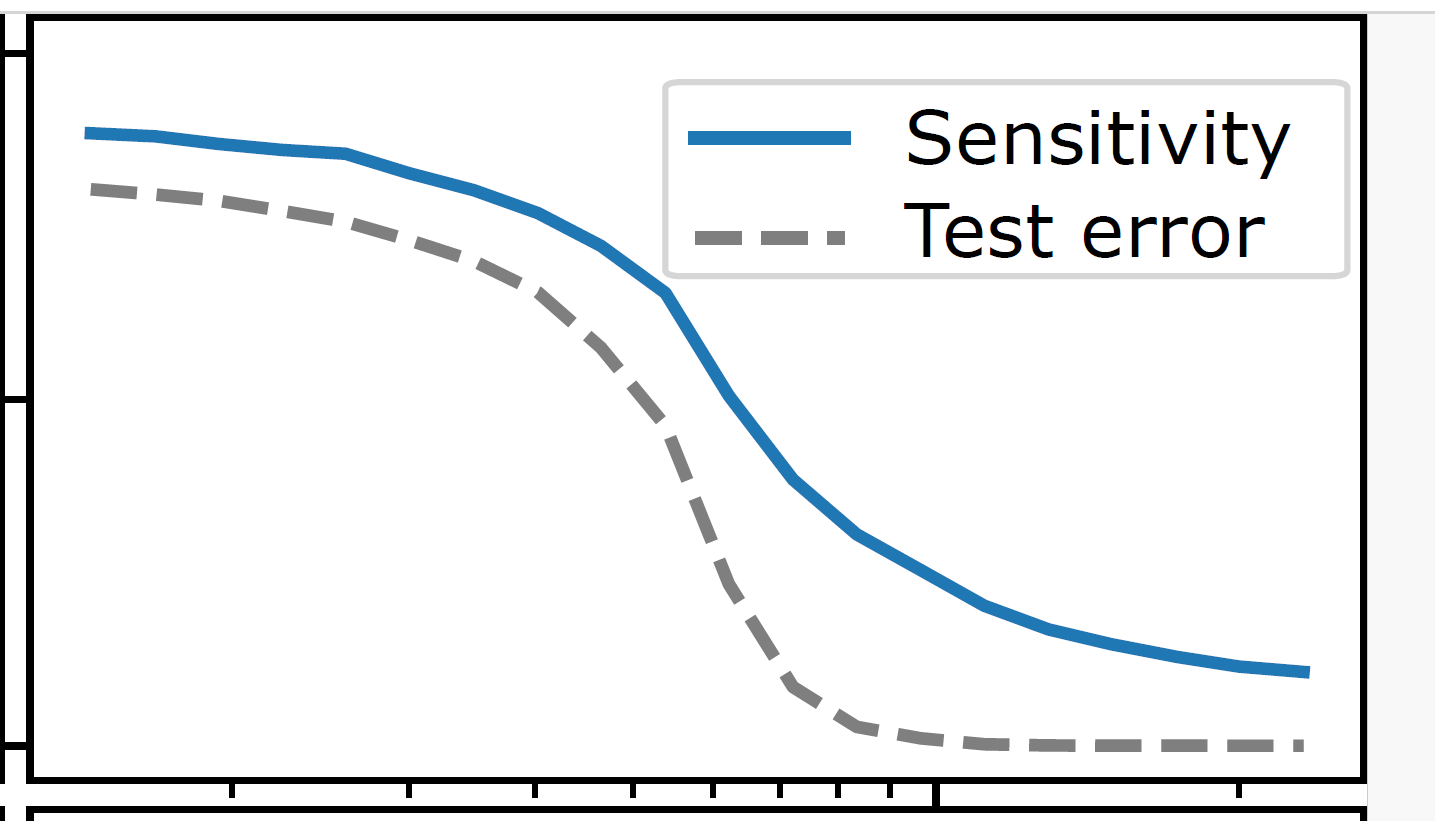
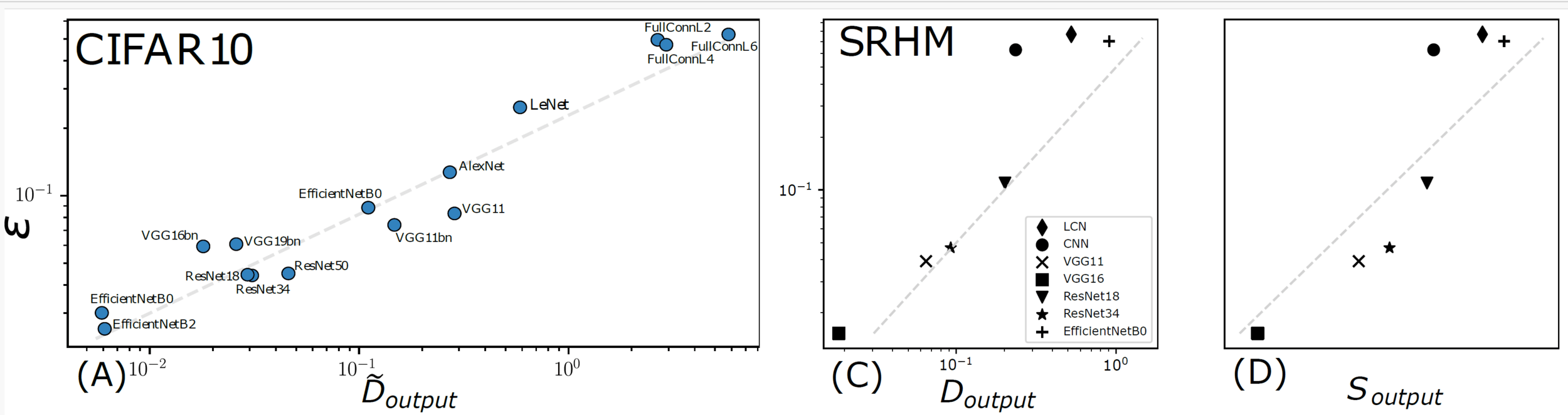
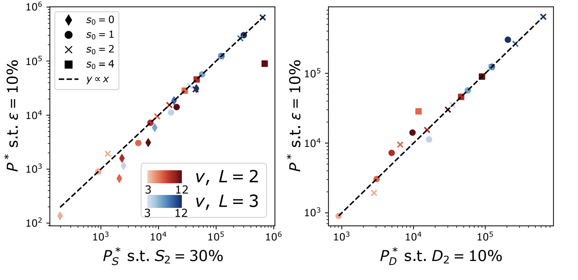
Capturing correlation with performance
Analyzing this model:
- How many training points to learn the task?
- And to learn the insensitivity to diffeomorphisms?
Sensitivity to diffeo
Sensitivity to diffeo
Test error
22/28
Learning by detecting correlations
\(x_1\)
\(x_2\)
\(x_3\)
\(x_4\)
- Without sparsity: learning based on recognizing correlations between patches with synonyms and label.
- With sparsity: latent variables generate patches with synonyms, distorted with diffeo
- All these patches share the same correlation with the label.
- Such correlation can be used by the network to group patches when \(P>P^*\)
23/28
How many training points to detect correlations
- Without sparsity (\(s_0=0\)): \(P^*_0\sim n_c m^L\)
- With sparsity, a local weight sees a signal with probability \(p\).
- For Locally Connected Networks: \(p=(s_0+1)^{-L}\)
- Correlations synonyms-label diluted
\(\Rightarrow\)To recover the synonyms, a factor \(1/p\) more data:
\(P^*_{\text{LCN}}\sim (s_0+1)^L P^*_0\)
- Polynomial in the dimension
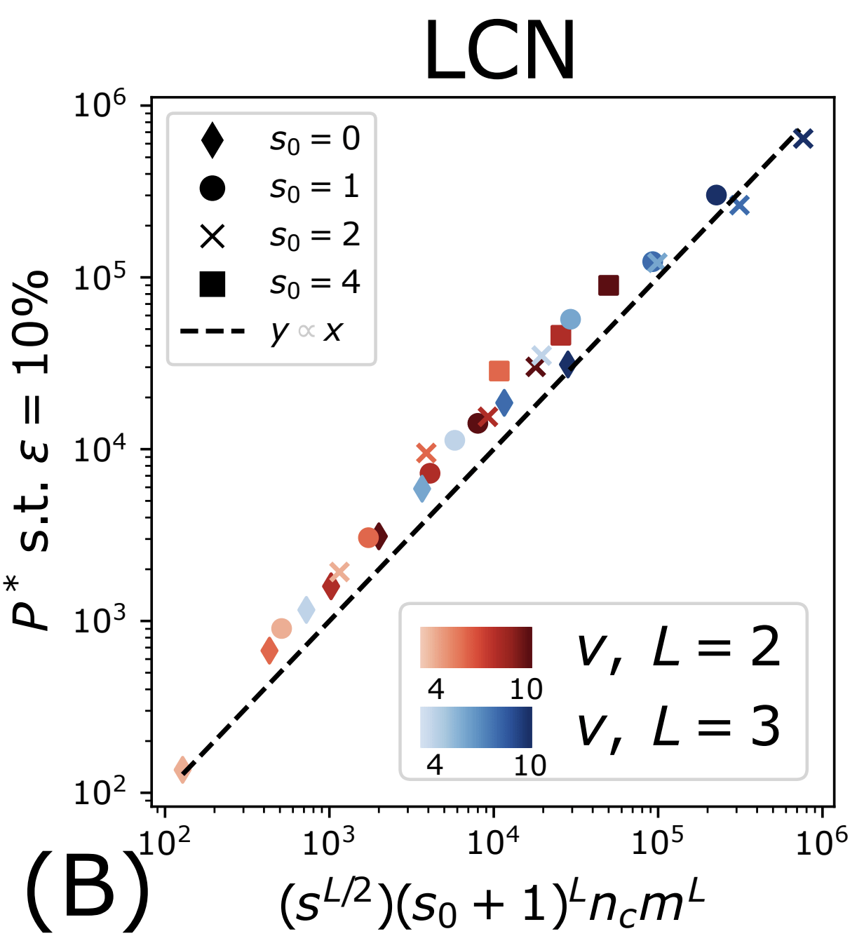
CNN: factor independent on \(L\)
24/28
What happens to Representations?
- To see a local signal (correlations), \(P^*\) data are needed
- For \(P>P^*\), the local signal is seen in each location it may end up
- The representations become insensitive to the exact location: insensitivity to diffeomorphisms.
- Both insensitivities are learnt at the same scale
\(x_1\)
\(x_2\)
\(x_3\)
\(x_4\)
25/28
Learning both insensitivities at the same scale \(P^*\)
Diffeomorphisms
learnt with the task
Synonyms learnt with the task
The hidden representations become insensitive to the invariances of the task
26/28
Takeaways
- Deep networks beat the curse of dimensionality on sparse hierarchical tasks.
- The hidden representations become insensitive to the invariances of the task: synonyms exchange and spatial local transformations.
- The more insensitive the network is, the better is its performance.
Test error
27/28
Future directions
Thank you!
- Extend the RHM to more realistic models of data (e.g. no fixed topology), and interpret how LLMs/Visual Models learn them.
- In the (S)RHM, learning synonyms and the task come together. To test this for real vision data, it is necessary to probe the hierarchical structure.
- Study the dynamics of learning the hierarchy in simple deep nets. Is there a separation of scales?
sofa
28/28
BACKUP SLIDES
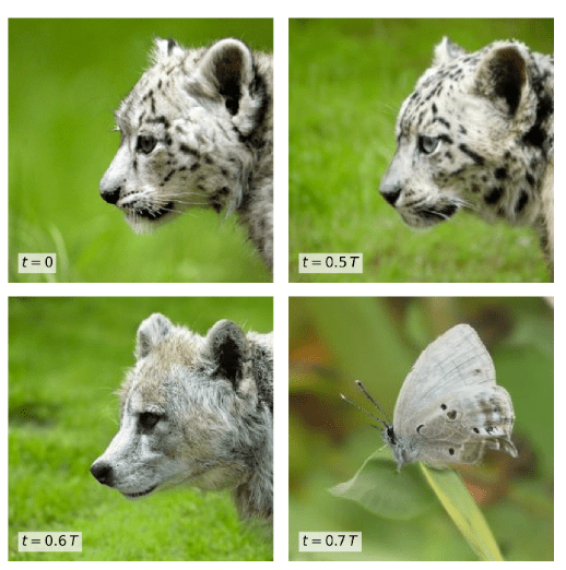
Measuring diffeomorphisms sensitivity
\(\tau(x)\)
\((x+\eta)\)
\(+\eta\)
\(\tau\)
\(f(\tau(x))\)
\(f(x+\eta)\)
\(x\)
Our model captures the fact that while sensitivity to diffeo decreases, the sensitivity to noise increases
Inverse trend
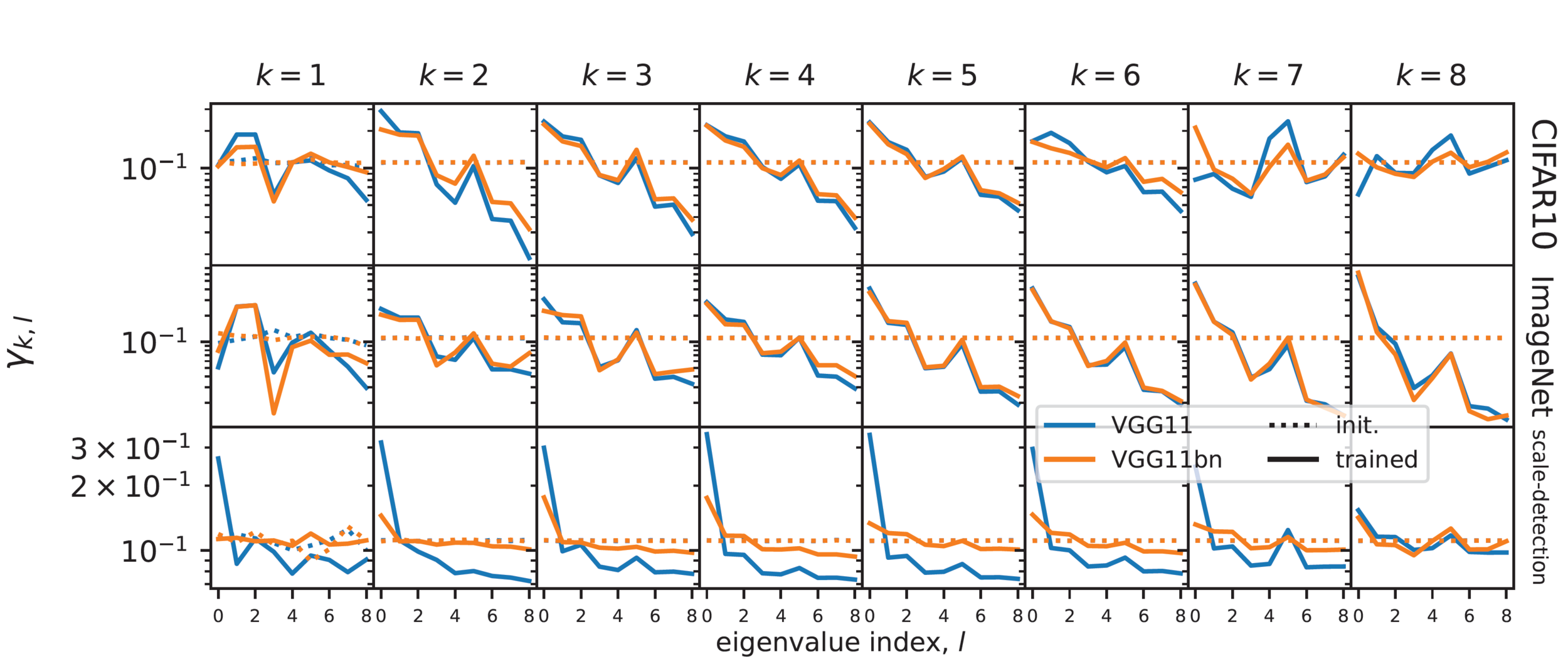
\(\gamma_{k,l}=\mathbb{E}_{c,c'}[\omega^k_{c,c'}\cdot\Psi_l]\)
- \(\omega^k_{c,c'}\): filter at layer \(k\) connecting channel \(c\) of layer \(k\) with channel \(c'\) of layer \(k-1\)
- \(\Psi_l\) : 'Fourier' base for filters, smaller index \(l\) is for more low-pass filters.
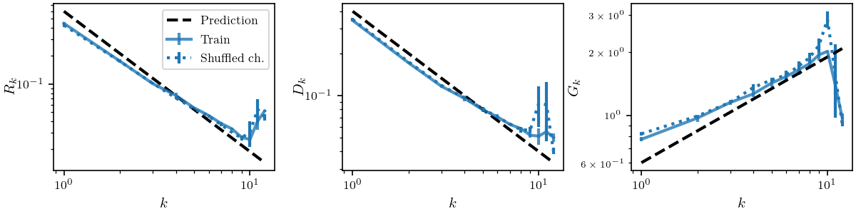
Frequency content of filters
Few layers become low-pass: spatial pooling
- Overall \(G_k\) increases
- Using odd activation functions as tanh nullifies this effect.
Noise
Increase of Sensitivity to Noise
Input
Avg Pooling
Layer 1
Layer 2
Avg Pooling
ReLU
\(G_k = \frac{\mathbb{E}_{x,\eta}\| f_k(x+\eta)-f_k(x)\|^2}{\mathbb{E}_{x_1,x_2}\| f_k(x_1)-f_k(x_2)\|^2}\)
- Difference before and after the noise: noise
- Concentrating average around positive mean
- Constant in depth \(k\)
- Difference of two peaks: one peak
- Squared norm decrease in \(k\)
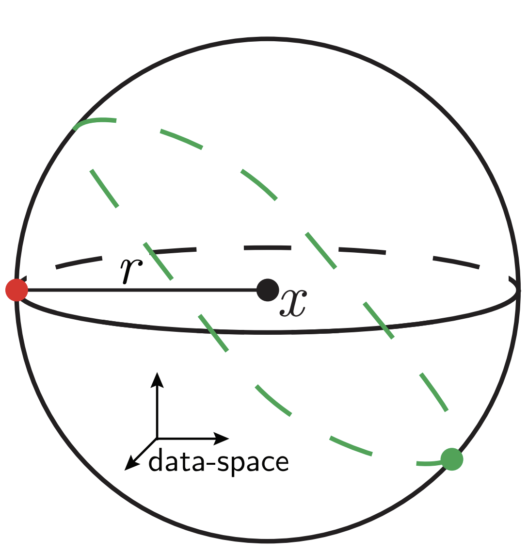
\(P^*\) points are needed to measure correlations
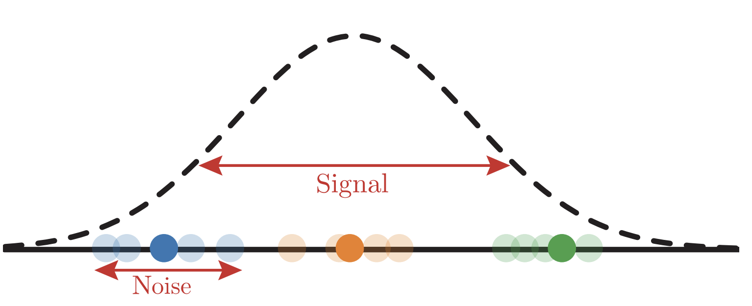
- If \(Prob(label|input\, patch)\) is \(1/n_c\): no correlations
- Signal: ratio std/mean of prob.
- Sampling noise: ratio std/mean of empirical prob
\(\sim[m^L/(mv)]^{-1/2}\)
\(\sim[P/(n_c m v)]^{-1/2}\)
Large \(m,\, n_c,\, P\):
\(P_{corr}\sim n_c m^L\)
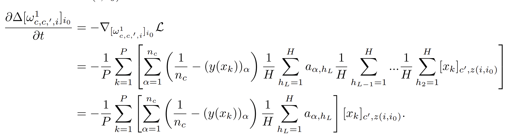
One GD step collapses
representations for synonyms
- Data: s-dimensional patches, one-hot encoding out of \(v^s\) possibilities (orthogonalization)
- Network: two-layer fully connected network, second layer Gaussian and frozen, first layer all 1s
- Loss: cross entropy
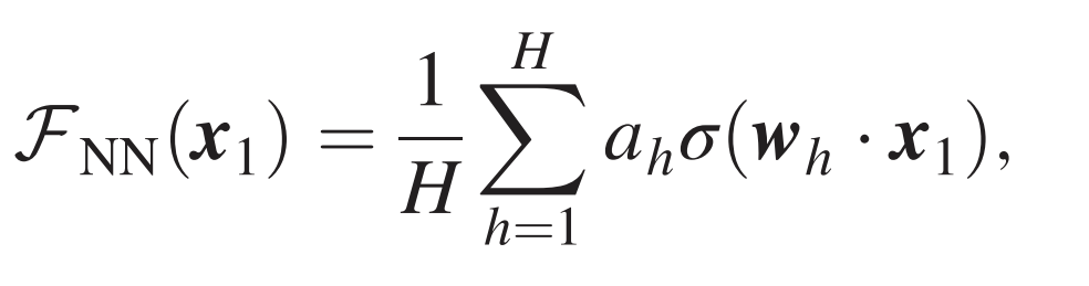
- Network learns the first composition rule of the RHM by building a representation invariant to exchanges of level-1 synonyms.
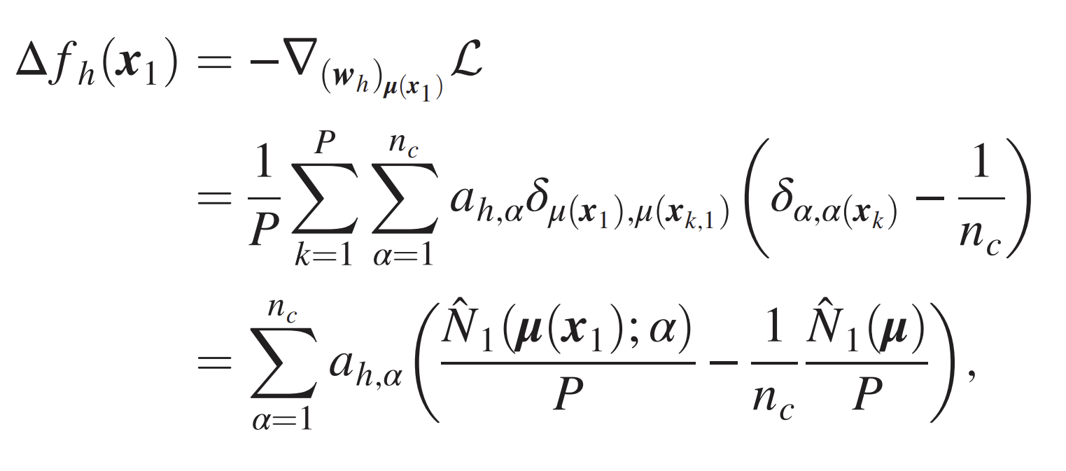
- One GD step: gradients \(\sim\) empirical counting of patches-label
- For \(P>P^*\) they converge to non-empirical, invariant for synonyms

Curse of Dimensionality without correlations
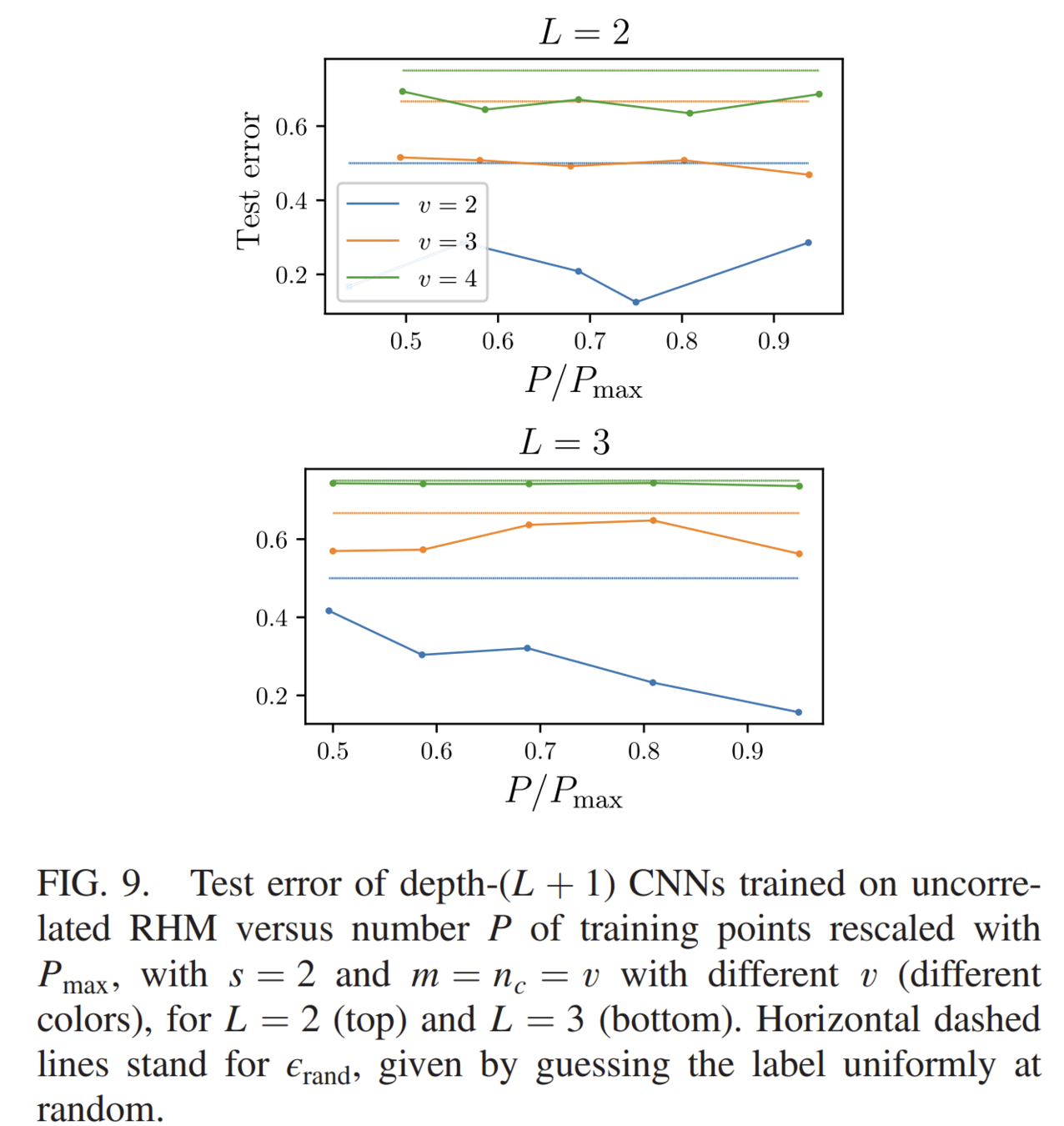
Uncorrelated version of RHM:
- features are uniformly distributed among classes.
- A tuple \(\mu\) in the \(j-\)th patch at level 1 belongs to a class \(\alpha\) with probability \(1/n_c\)
Curse of Dimensionality even for deep nets
Horizontal lines: random error
Which net do we use?
We consider a different version of a Convolutional Neural Network (CNN) without weight sharing
Standard CNN:
- local
- weight sharing
Locally Connected Network (LCN):
- local
weight sharing
One step of GD groups synonyms with \(P^*\) points
- Data: SRHM with \(L\) levels, with one-hot encoding of the \(v\) informative features, empty otherwise
- Network: LCN with \(L\) layers, readout layer Gaussian and frozen
- GD update of one weight at bottom layer depends on just one input position
- On average it is informative with \(p=(s_0+1)^{-L}\)
- Just a fraction of data points \(P'=p \cdot P\) contribute
- For \(P=(1/p) P^*_0\) the GD updates are as sparseless case with \(P^*_0\) points
- At that scale, a single step groups together representations with equal correlation with label
Single input feature!
The learning algorithm
- Regression of a target function \(f^*\) from \(P\) examples \(\{x_i,f^*(x_i)\}_{i=1,...,P}\).
- Interest in kernels renewed by lazy neural networks
f_P(x)=\sum_{i=1}^P a_i K(x_i,x)
\text{min}\left[\sum\limits_{i=1}^P\left|f^*(x_i)-f_P(x_i)\right|^2 +\lambda ||f_P||_K^2\right]
Train loss:
\(K(x,y)=e^{-\frac{|x-y|}{\sigma}}\)
E.g. Laplacian Kernel
- Kernel Ridge Regression (KRR):
Fixed Features
Failure and success of Spectral Bias prediction..., [ICML22]
- Key object: generalization error \(\varepsilon_t\)
- Typically \(\varepsilon_t\sim P^{-\beta}\), \(P\) number of training data
Predicting generalization of KRR
[Canatar et al., Nature (2021)]
General framework for KRR
- Predicts that KRR has a spectral bias in its learning:
\(\rightarrow\) KRR learns the first \(P\) eigenmodes of \(K\)
\(\rightarrow\) \(f_P\) is self-averaging with respect to sampling
- Obtained by replica theory
- Works well on some real data for \(\lambda>0\)
\(\rightarrow\) what is the validity limit?
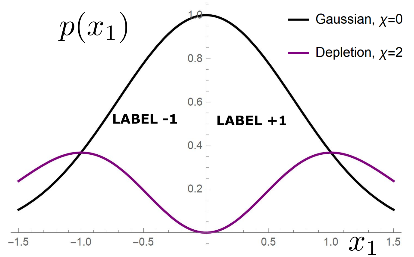
Our toy model
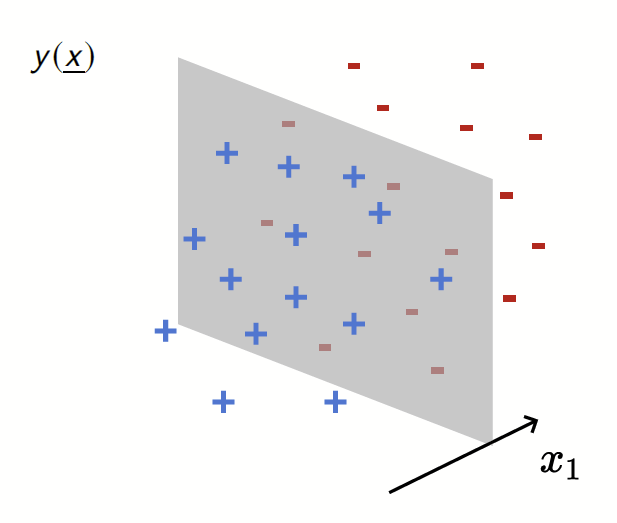
Depletion of points around the interface
p(x_1)= \frac{1}{\mathcal{Z}}\color{red}{|x_1|^\chi}\color{black} e^{-x_1^2}
Data: \(x\in\mathbb{R}^d\)
Label: \(f^*(x_1,x_{\bot})=\text{sign}[x_1]\)
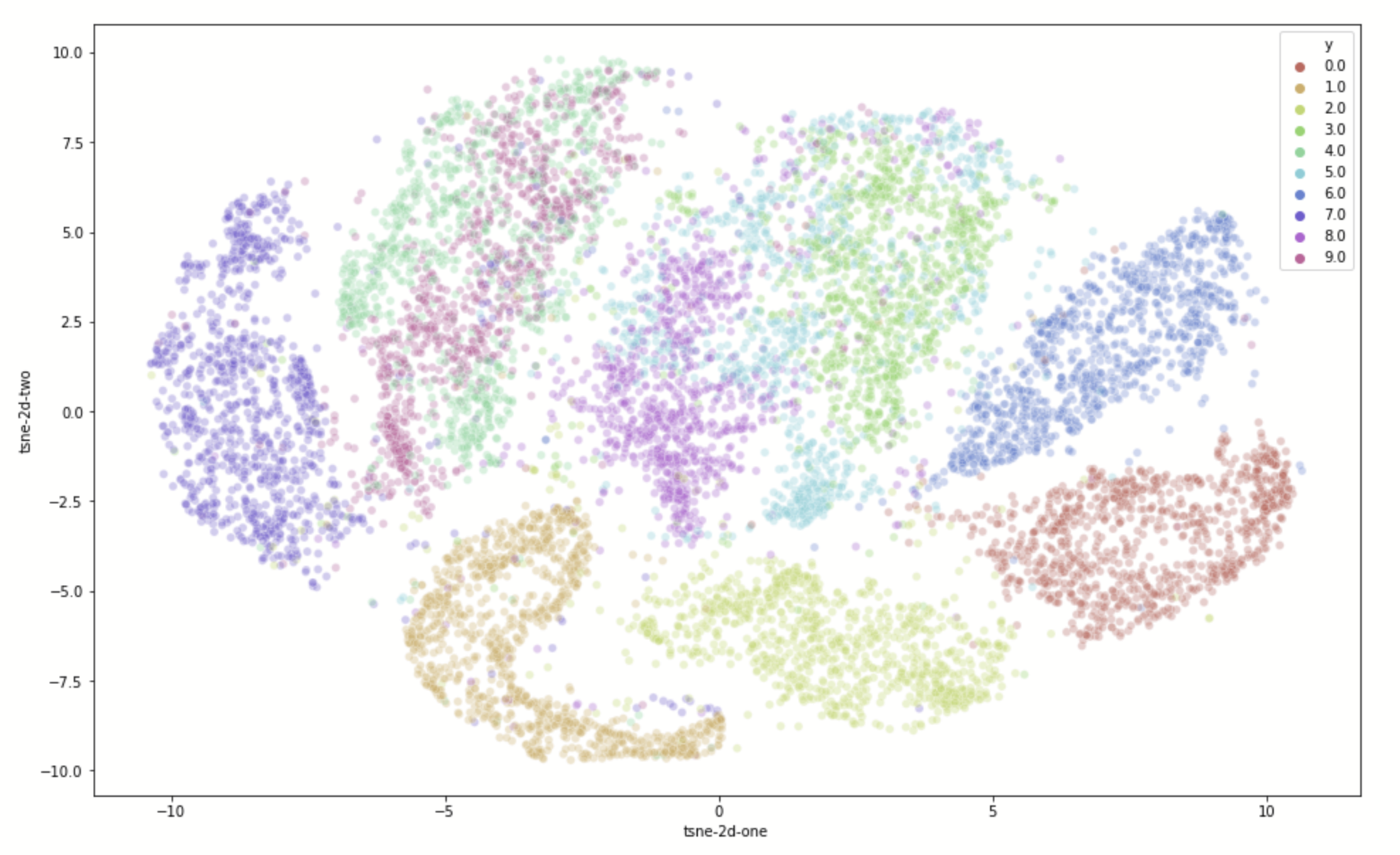
Motivation:
evidence for gaps between clusters in datasets like MNIST
Predictor in the toy model
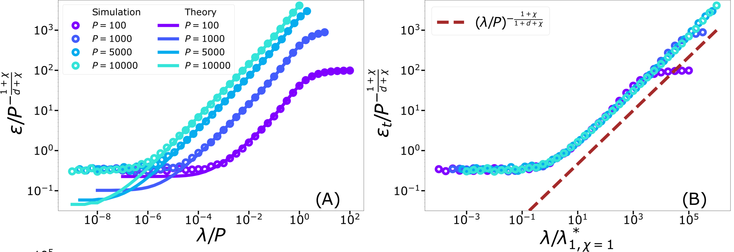
(1) Spectral bias predicts a self-averaging predictor controlled by a characteristic length \( \ell(\lambda,P) \propto \lambda/P \)
For fixed regularizer \(\lambda/P\):
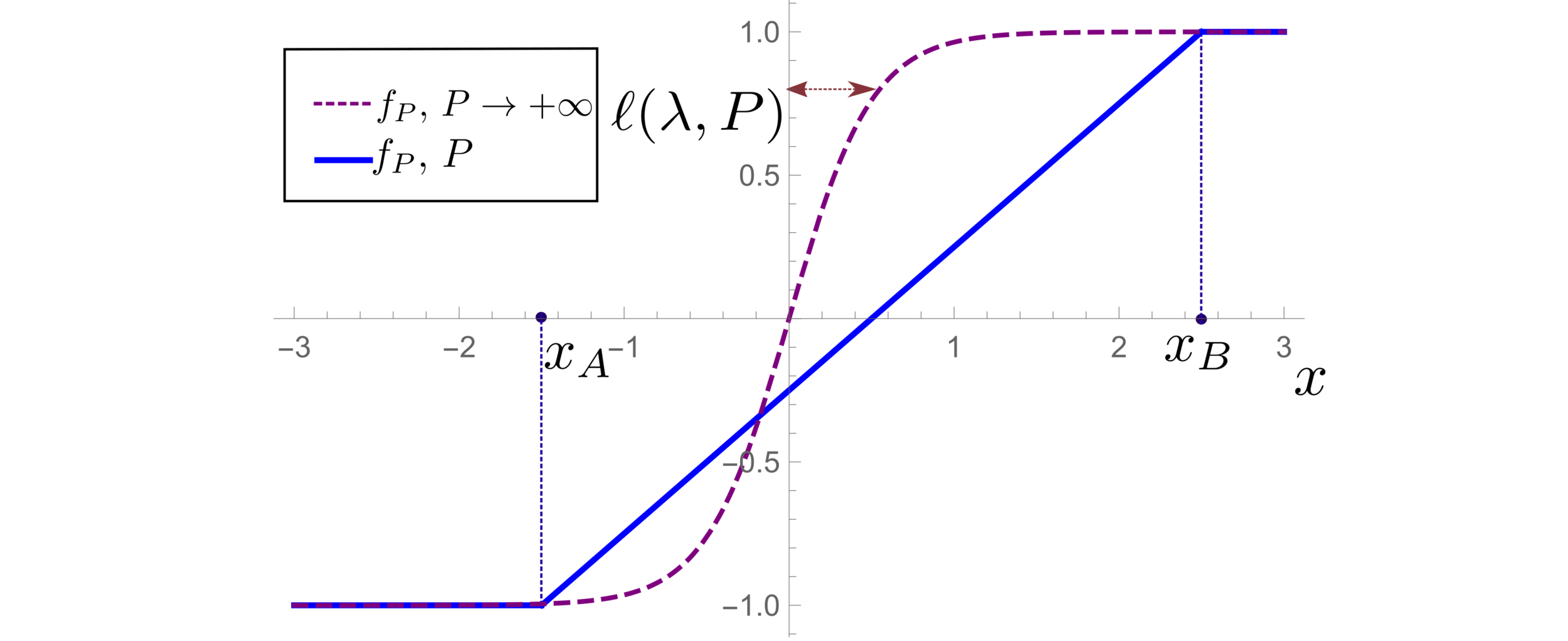
(2) When the number of sampling points \(P\) is not enough to probe \( \ell(\lambda,P) \):
- \(f_P\) is controlled by the statistics of the extremal points \(x_{\{A,B\}}\)
- spectral bias breaks down.
\(d=1\)
\varepsilon_B \sim P^{-(1+\frac{1}{d})\frac{1+\chi}{1+d+\chi}}
\varepsilon_t \sim P^{-\frac{1+\chi}{d+\chi}}
\neq
Different predictions for
\(\lambda\rightarrow0^+\)
- For \(\chi=0\): equal
- For \(\chi>0\): equal for \(d\rightarrow\infty\)
\lambda^*_{d,\chi}\sim P^{-\frac{1}{d+\chi}}
Crossover at:
\(\lambda\)
Spectral bias failure
Spectral bias success
Takeaways and Future directions
For which kind of data spectral bias fails?
Depletion of points close to decision boundary
Still missing a comprehensive theory for
KRR test error for vanishing regularization
Test error: 2 regimes
For fixed regularizer \(\lambda/P\):
\(\rightarrow\) Predictor controlled by extreme value statistics of \(x_B\)
\(\rightarrow\) Not self-averaging: no replica theory
(2) For small \(P\): predictor controlled by extremal sampled points:
\(x_B\sim P^{-\frac{1}{\chi+d}}\)
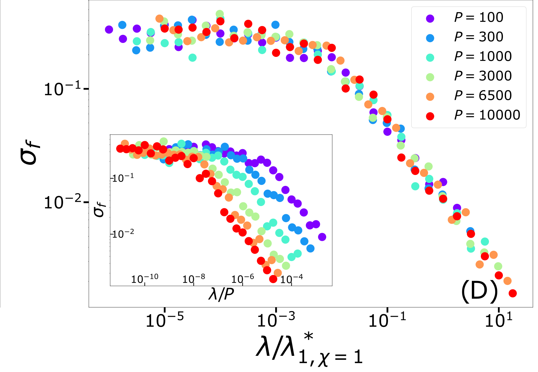
The self-averageness crossover
\(\rightarrow\) Comparing the two characteristic lengths \(\ell(\lambda,P)\) and \(x_B\):
\lambda^*_{d,\chi}\sim P^{-\frac{1}{d+\chi}}
\sigma_f = \langle [f_{P,1}(x_i) - f_{P,2}(x_i)]^2 \rangle
\varepsilon_B \sim P^{-(1+\frac{1}{d})\frac{1+\chi}{1+d+\chi}}
\varepsilon_t \sim P^{-\frac{1+\chi}{d+\chi}}
\neq
Different predictions for
\(\lambda\rightarrow0^+\)
- For \(\chi=0\): equal
- For \(\chi>0\): equal for \(d\rightarrow\infty\)
- Replica predictions works even for small \(d\), for large ridge.
- For small ridge: spectral bias prediction, if \(\chi>0\) correct just for \(d\rightarrow\infty\).
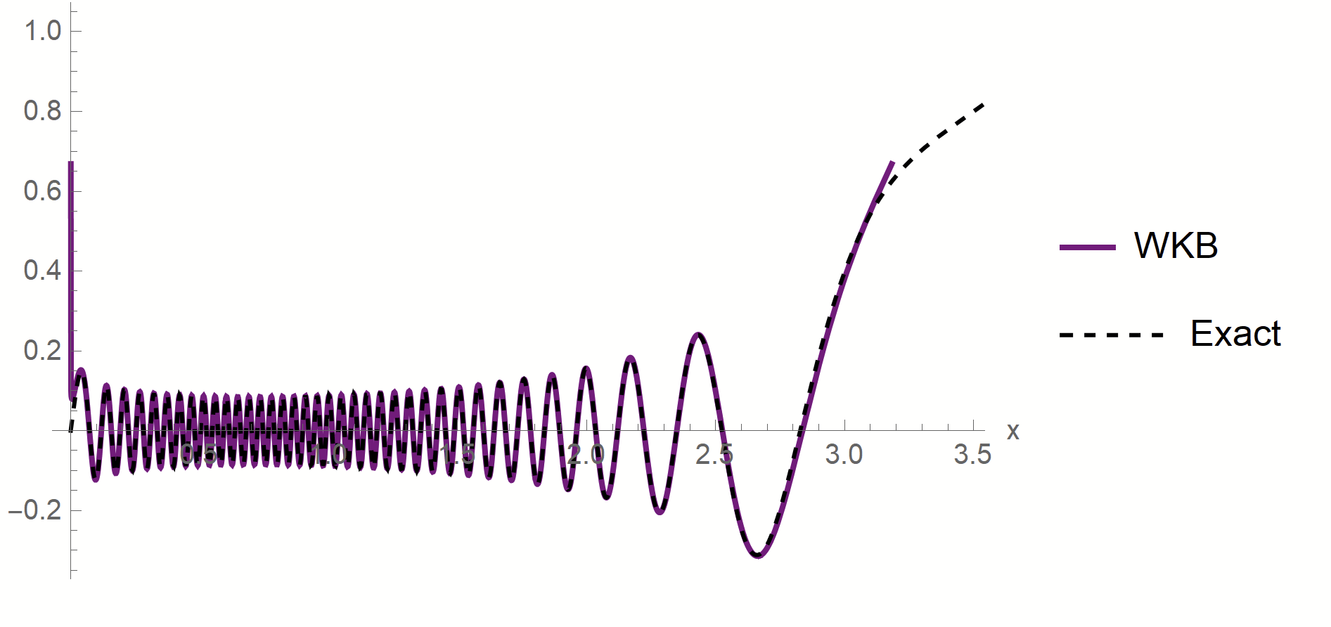
- To test spectral bias, we solved eigendecomposition of Laplacian kernel for non-uniform data, using quantum mechanics techniques (WKB).
- Spectral bias prediction based on Gaussian approximation: here we are out of Gaussian universality class.
Technical remarks:
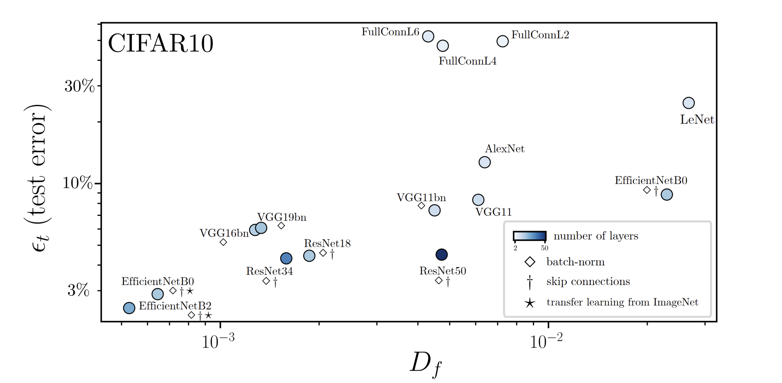
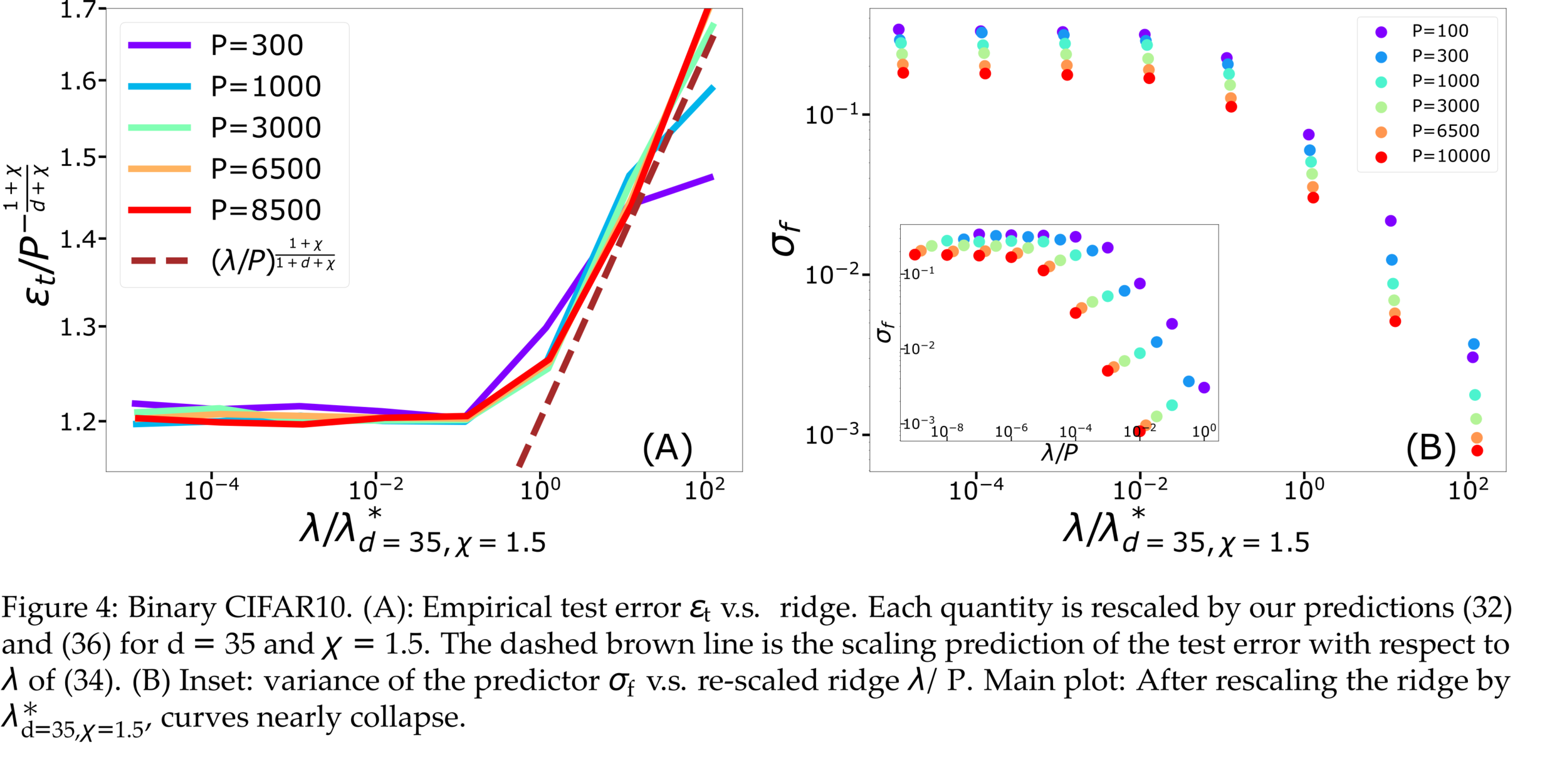
Fitting CIFAR10
Proof:
- WKB approximation of \(\phi_\rho\) in [\(x_1^*,\,x_2^*\)]:
\(\phi_\rho(x)\sim \frac{1}{p(x)^{1/4}}\left[\alpha\sin\left(\frac{1}{\sqrt{\lambda_\rho}}\int^{x}p^{1/2}(z)dx\right)+\beta \cos\left(\frac{1}{\sqrt{\lambda_\rho}}\int^{x}p^{1/2}(z)dx\right)\right]\)
x_1^*
x_2^*
- MAF approximation outside [\(x_1^*,\,x_2^*\)]
\(x_1*\sim \lambda_\rho^{\frac{1}{\chi+2}}\)
\(x_2*\sim (-\log\lambda_\rho)^{1/2}\)
- WKB contribution to \(c_\rho\) is dominant in \(\lambda_\rho\)
- Main source WKB contribution:
first oscillations
Formal proof:
- Take training points \(x_1<...<x_P\)
- Find the predictor in \([x_i,x_{i+1}]\)
- Estimate contribute \(\varepsilon_i\) to \(\varepsilon_t\)
- Sum all the \(\varepsilon_i\)
Characteristic scale of predictor \(f_P\), \(d=1\)
\sigma^2 \partial_x^2 f_P(x) =\left(\frac{\sigma}{\lambda/P}p(x)+1\right)f_P(x)-\frac{\sigma}{\lambda/P}p(x)f^*(x)
Minimizing the train loss for \(P \rightarrow \infty\):
\(\rightarrow\) A non-homogeneous Schroedinger-like differential equation
\(\rightarrow\) Its solution yields:
\ell(\lambda,P)\sim \left(\frac{\lambda\sigma}{P}\right)^{\frac{1}{(2+\chi)}}
Characteristic scale of predictor \(f_P\), \(d>1\)
- Let's consider the predictor \(f_P\) minimizing the train loss for \(P \rightarrow \infty\).
f_P(x)=\int d^d\eta \frac{p(\eta) f^*(\eta)}{\lambda/P} G(x,\eta)
- With the Green function \(G\) satisfying:
\int d^dy K^{-1}(x-y) G_{\eta}(y) = \frac{p(x)}{\lambda/P} G_{\eta}(x) + \delta(x-\eta)
- In Fourier space:
\mathcal{F}[K](q)^{-1} \mathcal{F}[G_{\eta}](q) = \frac{1}{\lambda/P} \mathcal{F}[p\ G_{\eta}](q) + e^{-i q \eta}
- In Fourier space:
\mathcal{F}[K](q)^{-1} \mathcal{F}[G_{\eta}](q) = \frac{1}{\lambda/P} \mathcal{F}[p\ G_{\eta}](q) + e^{-i q \eta}
\begin{aligned}
\mathcal{F}[G](q)&\sim q^{-1-d}\ \ \ \text{for}\ \ \ q\gg q_c\\
\mathcal{F}[G](q)&\sim \frac{\lambda}{P}q^\chi\ \ \ \text{for}\ \ \ q\ll q_c\\
\text{with}\ \ \ q_C&\sim \left(\frac{\lambda}{P}\right)^{-\frac{1}{1+d+\chi}}
\end{aligned}
- Two regimes:
- \(G_\eta(x)\) has a scale:
\ell(\lambda,P)\sim 1/q_c\sim \left(\frac{\lambda}{P}\right)^{\frac{1}{1+d+\chi}}
PhD_defense_diffeo_hierarchy_Long_CORRECTED
By umberto_tomasini


