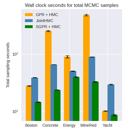
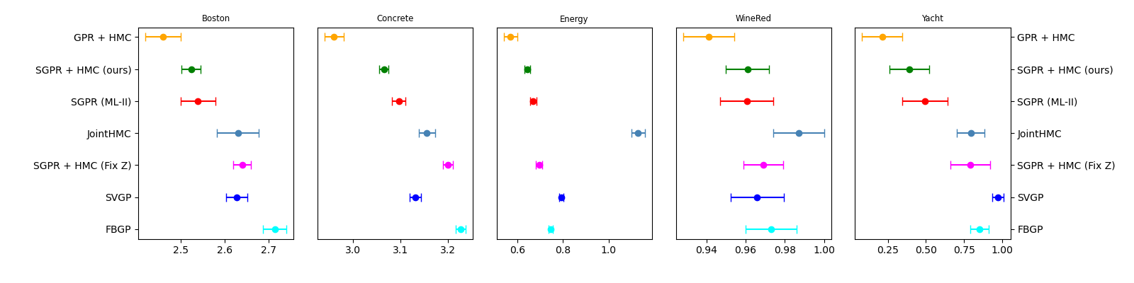
Sparse Gaussian Process Hyperparameters: Optimise or Integrate?

Vidhi Lalchand\(^{1}\), Wessel P. Bruinsma\(^{2}\), David R. Burt \(^{3}\), Carl E. Rasmussen\(^{1}\)

Motivation

  • This work centers on Bayesian hyperparameter inference in sparse Gaussian process regression.
  • Traditional gradient based optimisation (ML-II) can be extremely sensitive to starting values.
  • ML-II hyperparameter estimates are subject to high variability and underestimate prediction uncertainty.
  • We propose a novel and computationally efficient scheme for Fully Bayesian inference in sparse GPs.

University of Cambridge\(^{1}\), Microsoft Research A14 Science \(^{2}\), MIT LIDS \(^{3}\)

\begin{aligned} \textrm{Approach}\hspace{4mm} & \textrm{Time/it.} & \textrm{Mem./it.} & \hspace{4mm} \textrm{Param / Vars} \\ \textrm{Non-collapsed }\hspace{4mm} & \hspace{4mm}\textcolor{darkgreen}{m^3} & \textcolor{darkgreen}{m^2} \hspace{4mm}& \hspace{6mm}\textcolor{orange}{n_\theta + m}\\ \textrm{Collapsed \textcolor{blue}{(ours)}}\hspace{4mm} & \hspace{4mm}\textcolor{orange}{nm^2} & \textcolor{darkgreen}{m^2} \hspace{4mm}& \hspace{6mm}\textcolor{darkgreen}{n_\theta} \\ \end{aligned}
y_n = f(x_n) + \epsilon_n, \, \, \epsilon_n \sim \mathcal{N}(0, \sigma^2), \, f \sim \mathcal{GP}(0, k_{\theta})
\log p(\bm{y}|\bm{\theta}) = \log \int p(\bm{y}|f)p(f|\bm{\theta})df = c \smash{ \underbrace{-\tfrac{1}{2}\bm{y}^{T} (K_{\theta} + \sigma^{2}I)^{-1} \bm{y}}_{\textrm{data fit term}} - \underbrace{\tfrac{1}{2}|K_{\theta} + \sigma^{2}I|}_{\textrm{complexity penalty}} }
f \sim \mathcal{GP}(0, k_{\bm{\theta}})
\bm{y} = (y_{n})_{n=1}^{N} \subseteq \mathbb{R}
X = (\bm{x}_{n})_{n=1}^{N} \subseteq \mathbb{R}^D
p(\bm{y}|f) = \prod_{n=1}^{N}\mathcal{N}(y_{n}|f_{n}, \sigma^2)
\bm{u} = \{f(\bm{z}_m)\}_{m=1}^{M} \subseteq \mathbb{R}
Z = \{\bm{z}_{m}\}_{m=1}^{M}, \bm{z}_m \in \mathbb{R}^{D}
Inputs / Outputs
Latent function prior
Inducing locations
Inducing variables

Overall, the core training algorithm alternates between two steps:


By sampling from \( q^{*}(\bm{\theta})\), we side-step the need to sample from the joint \( (\bm{u},\bm{\theta})\)-space yielding a significantly more efficient algorithm in the case of regression with a Gaussian likelihood.

\begin{aligned} &\textrm{1. Sampling step for $\theta$:} \hspace{2mm} \theta_{j} \sim q^{\ast}(\theta) \propto \mathcal{L}({\bm{\theta}, Z_{opt}}) + \log p(\bm{\theta}), \hspace{2mm}\textcolor{orange}{[\textrm{Keep $Z_{opt}$ fixed}]}\\ &\textrm{2. Optimisation step for $Z$:} \hspace{2mm} Z_{opt} \longleftarrow \texttt{optim}(\mathcal{\hat{L}}), \textrm{where} \\ & \hspace{5mm} \mathcal{\hat{L}} = \mathbb{E}_{q^{\ast}(\theta)}[\mathcal{L}(\theta, Z)] \approx \dfrac{1}{J}\sum_{j=1}^{J}\mathcal{L}(\theta_{j}, Z_{opt}), \hspace{2mm}\textcolor{orange}{[\textrm{Keep $\theta$ fixed}]}\end{aligned}
\bm{\theta}^* \in {\textstyle\argmax_{\bm{\theta},Z}}\, \mathcal{L}_{\bm{\theta},Z}.
Hyperparameter inference:
p(f, \bm{u} | \bm{y}, {\bm{\theta}}) \approx q(f, \bm{u} | {\bm{\theta}}) = p(f | \bm{u}, {\bm{\theta}}) q(\bm{u})
Variational approximation:

Canonical Inference

"Doubly Collapsed" Inference

p(f, \bm{u}, \bm{\theta}| \bm{y}) \approx q(f, \bm{u}, {\bm{\theta}}) = p(f | \bm{u}, {\bm{\theta}}) q(\bm{u}|\bm{\theta})q(\bm{\theta})
\begin{aligned} \log p(\bm{y}) &\geq \int q(\bm{\theta}) \mathcal{L}_{\bm{\theta}, Z}d\bm{\theta} - \textrm{KL}(q(\bm{\theta}) || p(\bm{\theta})) \\ &= \int q(\bm{\theta})\log \dfrac{M_{\theta,Z}p(\bm{\theta})}{q(\bm{\theta})} d\bm{\theta} =: \mathcal{L}^{*}_Z(q(\bm{\theta})),\\ \mathcal{L}^*_Z(q(\bm{\theta})) &= \log C_Z - \textrm{KL}(q(\bm{\theta}) || q^{*}(\bm{\theta})) \end{aligned}
\textrm{where, } q^{*}(\bm{\theta}) = M_{\bm{\theta},Z}p(\bm{\theta})/ C_Z
Variational approximation:
\frac{\text{d}}{\text{d} Z} \mathcal{L}^{**}_{Z} %(q^*_{\bm{\phi}}) = \left.\frac{\partial}{\partial Z} \mathcal{L}^{*}_{Z}(q) %(q^*_{\bm{\phi}}) \right|_{q=q^*(\bm{\theta})} + \left\langle \cancel{ \left.\frac{\delta}{\delta q} \mathcal{L}^{*}_{Z}(q)\right|_{q=q^*(\bm{\theta})} } , \frac{\partial}{\partial Z} q^*(\bm{\theta}) \right\rangle \approx \frac1J \sum_{j=1}^J \frac{\partial}{\partial Z} %\left( \mathcal{L}_{\bm{\theta}_j, Z} % + \log p(\bm{\theta}_j) % \right)

Gradients of the doubly collapsed ELBO 

Mathematical set-up

/

Sparse GP poster

By Vidhi Lalchand

Sparse GP poster

  • 20