Permutation Invariant Multi-Output Gaussian processes

Vidhi Lalchand

22nd November 2024

for Cancer Dose Response Surface Modelling

The multi-output setting

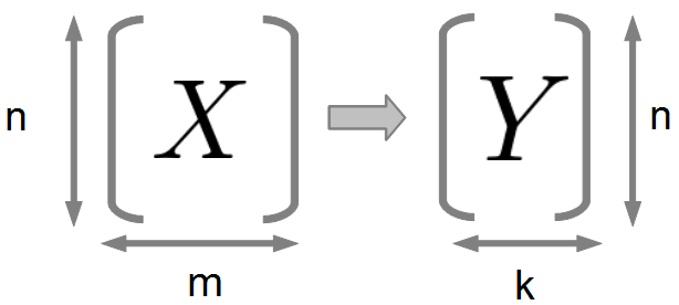
Predicting two or more output variables $\mathbf{y} = [y_1, y_2, \dots, y_k]$ simultaneously from some high-dimensional input $\mathbf{x}$.

These outputs are typically interdependent and correspond to the same overarching task. For instance, predicting multiple attributes of a car (e.g., make, model, and year) given an image of the car.

Formally, you can write down the model:

$f(\mathbf{x}; \theta) = \hat{\mathbf{y}} = [\hat{y}_1, \hat{y}_2, \dots, \hat{y}_k]$

Where:
- $\mathbf{x}$ is the input.
- $\theta$ are the parameters of the model.
- $\hat{\mathbf{y}} = [\hat{y}_1, \hat{y}_2, \dots, \hat{y}_k]$ are the predicted outputs.

$N$

$D$

$K$

Outputs depend on the input and each other:

y_i = f_i(\mathbf{x}, \mathbf{y}_{-i}; \theta_i)

p(\mathbf{y} \mid \mathbf{x}; \theta) \neq \prod_{i=1}^k p(y_i \mid \mathbf{x}; \theta)

Joint data likelihood doesn't admit this factorisation:

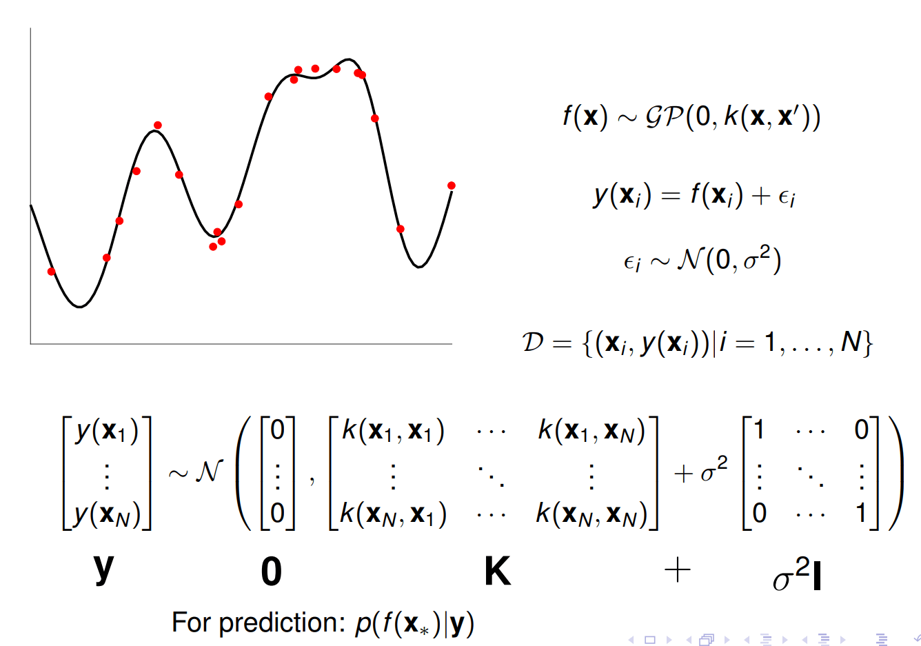
Single-output Gaussian processes

GPs are flexible prior over functions parameterised by a kernel function.

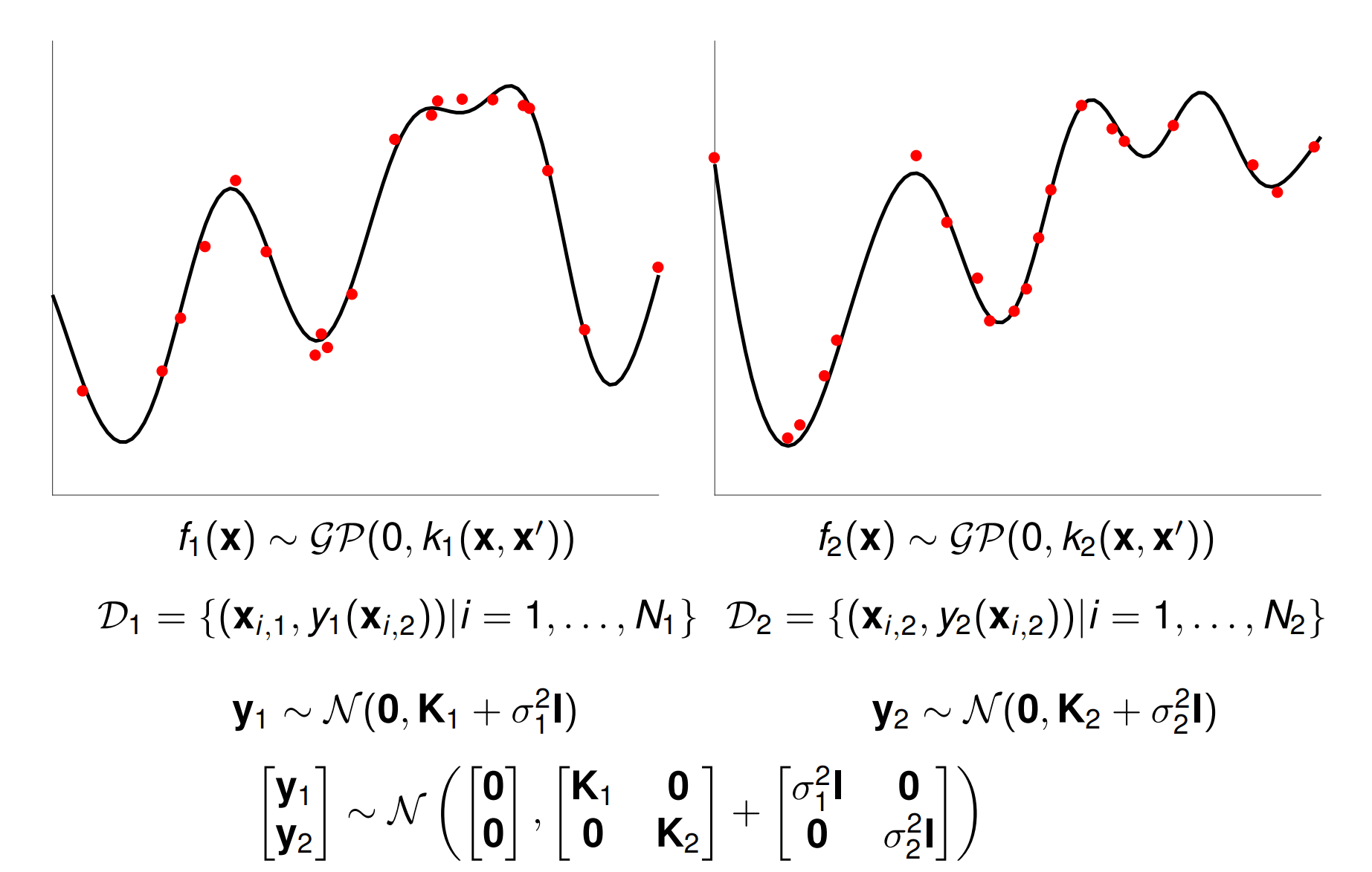
Single-output Gaussian processes $\rightarrow$ Multi-output Gaussian processes

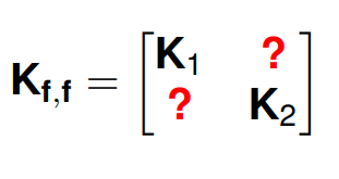
Main challenge:

Introduce dependencies between the outputs. Tantamount to learning the cross-covariance blocks.

Parametrising Multi-output Gaussian processes

Intrinsic model of coregionalisation (IMC)

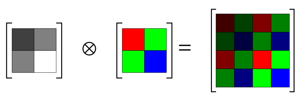
You can model the interaction between the outputs using a coregionalisation matrix $\mathbf{B}$ and use a shared covariance $\mathbf{K}$ that drives both outputs $f_{1}(\mathbf{x})$ and $f_{2}(\mathbf{x})$.

The interaction between the outputs is given by a positive semi-definite matrix $\mathbf{B}$. In the two output case, it is give by,

\mathbf{B} = \begin{bmatrix} b_{11} & b_{12} \\ b_{21} & b_{22} \\ \end{bmatrix}

\begin{bmatrix} \mathbf{f}_{1} \\ \mathbf{f}_{2} \end{bmatrix} = \begin{bmatrix} f_1(\mathbf{x}_1) \\ \vdots \\ f_1(\mathbf{x}_N) \\ f_2(\mathbf{x}_1) \\ \vdots \\ f_2(\mathbf{x}_N) \end{bmatrix} \sim \mathcal{N}\left( \begin{bmatrix} 0 \\ 0 \end{bmatrix}, \mathbf{B} \otimes \mathbf{K} \right)

\begin{bmatrix} b_{11}\mathbf{K} & b_{12}\mathbf{K} \\ b_{21}\mathbf{K} & b_{22}\mathbf{K} \\ \end{bmatrix}_{2N \times 2N}

2 \times 2

4 \times 4

WW^{T}

(to ensure psd)

Another way to think about $ \mathbf{B}$ is as capturing inter-output covariance through an output based kernel function.

k\left([\mathbf{x}, i], [\mathbf{x}',j] \right) = k_{\text{inputs}}(\mathbf{x}, \mathbf{x}')\cdot k_{\text{outputs}}(i, j)

\mathbf{K} = \mathbf{K}_{\text{inputs}} \otimes \mathbf{K}_{\text{outputs}}

N \times N

M \times M

MN \times MN

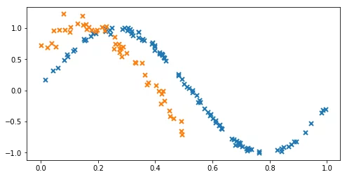
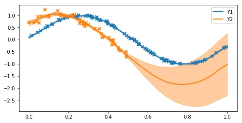
Intrinsic model of coregionalisation: Synthetic example

\begin{aligned} y_1 &= \sin(6x) + \epsilon_1, \quad \epsilon_1 \sim \mathcal{N}(0, 0.009), \\ y_2 &= \sin(6x + 0.7) + \epsilon_2, \quad \epsilon_2 \sim \mathcal{N}(0, 0.01). \end{aligned}

y_{1} / y_{2}

The model does a reasonable job of estimating the noise variance and the lengthscale. The posterior variance is higher on the second output where there is no training data.

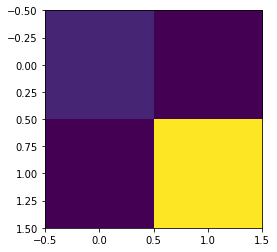
B = \begin{bmatrix} 3.10552 & 2.9025 \\ 2.9025 & 4.83607 \end{bmatrix}

Diagonal Elements $B [i, i]$ : Represent the variance of the $i$ -th output. Larger values indicate higher variability in that output.
Off-Diagonal Elements $B [i, j]$ : Represent the covariance between the $i$ -th and $j$ -th outputs. Positive values indicate that the outputs tend to increase or decrease together.

Parametrising Multi-output Gaussian processes

\mathbf{K}_{\text{joint}} = \mathbf{B} \otimes \mathbf{K}_{\text{input}}, \\ \mathbf{B} \in \mathbb{R}^{M \times M} \\ \ \mathbf{K}_{\text{input}} \in \mathbb{R}^{N \times N}

\mathbf{K}_{\text{joint}} = \sum_{k=1}^q \mathbf{B}_k \otimes \mathbf{K}_k,

$q$: Number of independent latent GPs.
$ \mathbf{B}_k = \mathbf{b}_k \mathbf{b}_k^\top \in \mathbb{R}^{M \times M} $: Rank-1 coregionalization matrix for the $k$-th latent GP.
$ \mathbf{b}_k \in \mathbb{R}^M $: Vector describing how the $k$-th latent GP contributes to each output.
$ \mathbf{K}_k \in \mathbb{R}^{N \times N} $: Covariance matrix of the $k$-th latent GP over the inputs.

"Intrinsic" model of coregionalisation:

"Linear" model of coregionalisation:

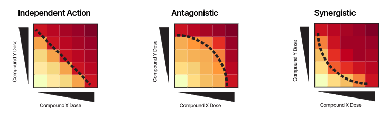
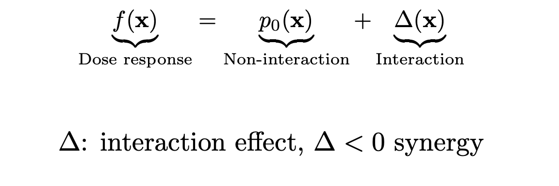
Drug-synergy modelling through dose-response surfaces

The nature of a drug combination, as synergistic, antagonistic or non-interacting, is usually studied by in-vitro dose–response experiments on cancer cell lines, through e.g. a cell viability assay.

https://theprismlab.org/white-papers/multiplexed-cancer-cell-line-combination-screening-using-prism

Combination therapies are routinely used in cancer care, as monotherapies are rarely effective.
However, which combinations would benefit cancer patients is largely unknown.
Studies that measure candidate combinations (of drugs) across many cancer cell lines simultaneously can help support combinations research [PRISM Lab].

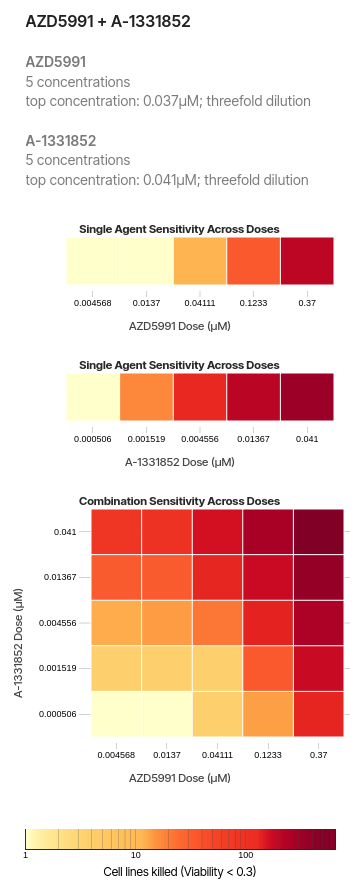
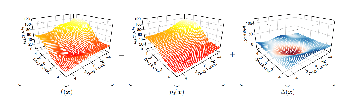
Drug-synergy modelling: Bliss model of independence

https://theprismlab.org/white-papers/multiplexed-cancer-cell-line-combination-screening-using-prism

The Bliss model assumes that the two drugs X and Y act independently to achieve their effects.

$E_A$ : The probability of drug $A$ killing a cell.
$E_B$ : The probability of drug $B$ killing a cell.
The probability of neither drug killing a cell is:
$E_A) \cdot (1 - E_B).$
Therefore, the expected viability $V_{XY}$ is, $VABV_{ABV$
$VAB=VA⋅VB,V_{AB} = V_A \cdot V_B,$

Observed Results:

If $Vobs=0.2V_{\text{obs}} = 0.2$ : Synergy (fewer cells survive than expected).
If $Vobs=0.3V_{\text{obs}} = 0.3$ : Additivity (matches expected survival).
If $Vobs=0.4V_{\text{obs}} = 0.4$ : Antagonism (more cells survive than expected).

$V_{X} = 0.5$ and $V_{Y} =0.6$

$V_{XY} = 0.3$

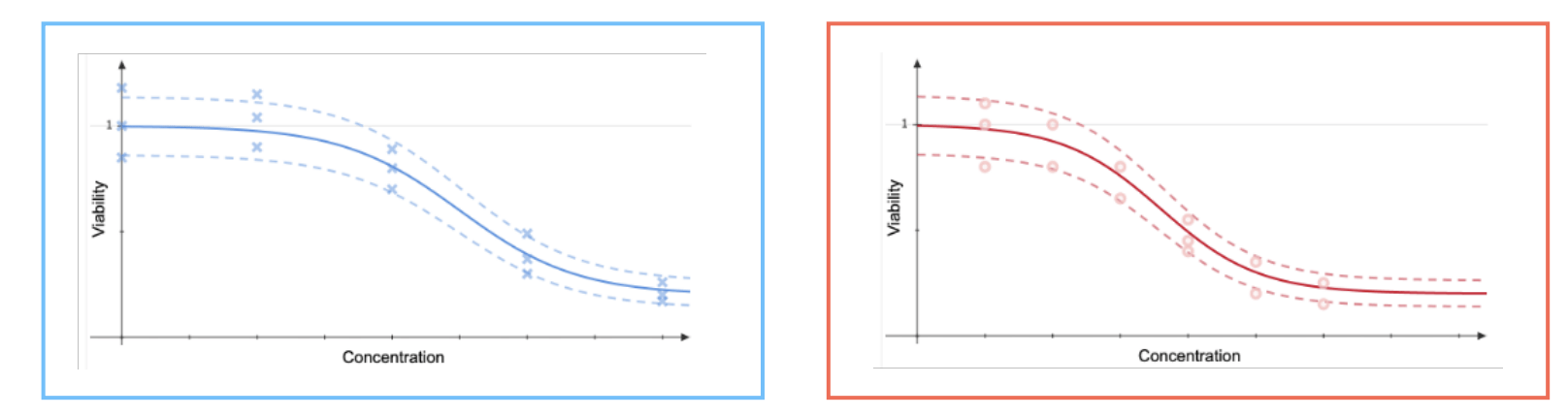
Drug-synergy modelling through dose-response surfaces

Bliss independence

Multi-output Gaussian process

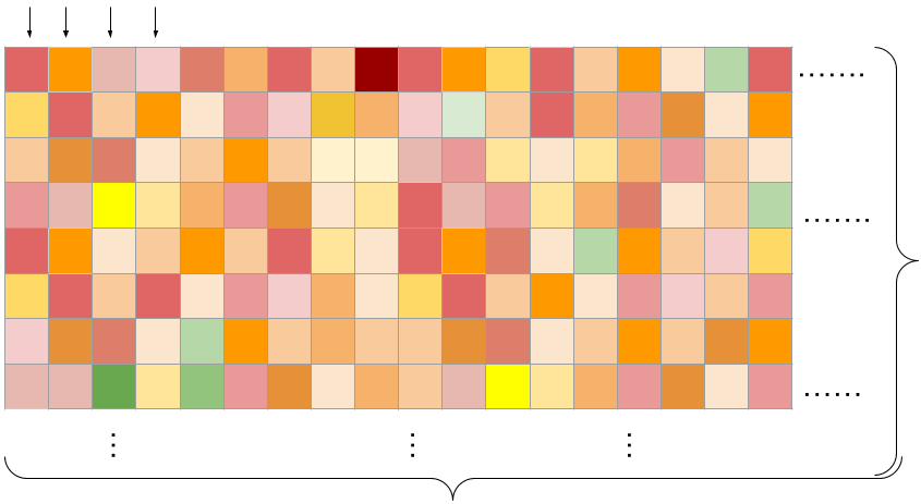
Understanding the training dataset

Built a model for the O'Neil (2016) dataset released by Merck Laboratories, Boston.

(c1, A, B)

(c2, A, B)

(c3, A, B)

(0, 0.11)

(0,0.22)

(0,0.33)

In this dataset, 38 drugs were combined in a pairwise manner into 583 distinct combinations that were screened on 39 cancer cell lines across 6 different tissues of origin (Lung, 8; Ovarian, 9; Melanoma, 6; Colon, 8; Breast, 6; Prostate, 2)

........

$N_{d}$ = 583

$N_{c}$ = 39

$N_{}$ = 100

No. of drug concentrations

No. of cancer cell lines

No. of drug pairs.

(1,1)

Caveat:

-In reality, the experiments are performed on different grids of concentrations,

- we scale the concentration ranges of each experiment to the unit box and constructed a common grid of concentrations.

O'Neil et al. (2016). An An Unbiased Oncology Compound Screen to Identify Novel Combination Strategies. Mol Cancer Ther. 2016 Jun;15(6):1155-62

$N_{}$

$N_{c} \times N_{d} = $ 22,737

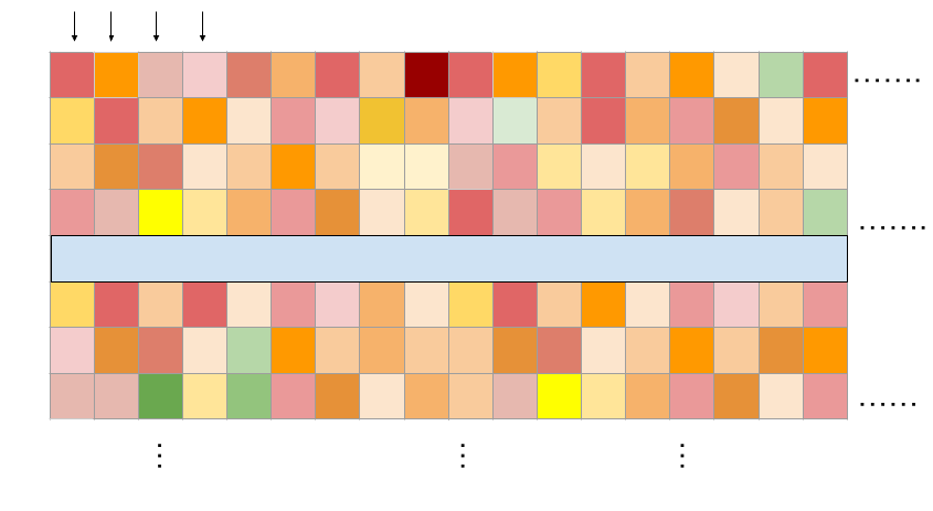
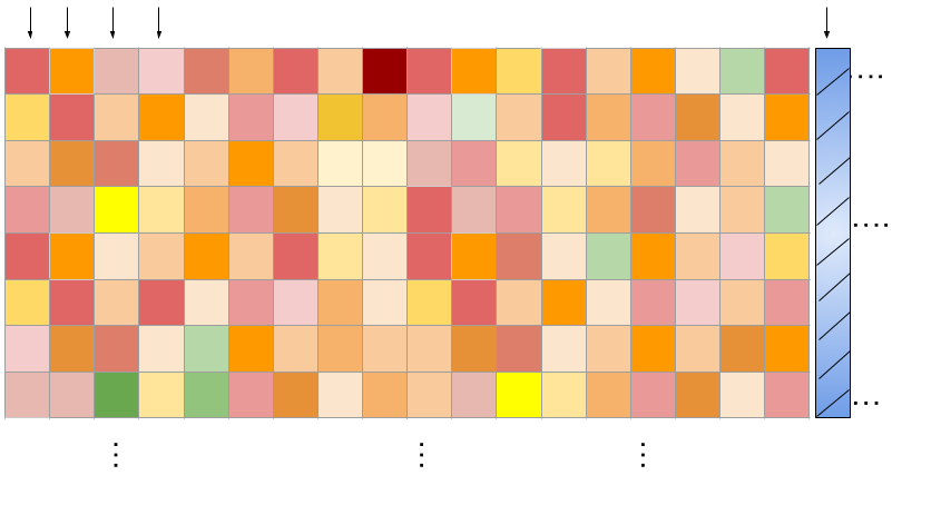
Each output column (experiment) corresponds to some measurements on a dose-response surface of a triplet $(c, A,B)$

f(\mathbf{x}) = p_{0}(\mathbf{x}) + \Delta(\mathbf{x})

Let $\mathbf{x} = (x_{1}, x_{2})$ denote drug concentrations for an arbitrary pair of drugs, then the dose-response function:

p_{0}(\mathbf{x}) = h_{1}(x_{1})h_{2}(x_{2})

\Delta(\mathbf{x}) = \zeta (g(\mathbf{x}))

g(.) \sim \mathcal{GP}(\mathbf{0}, k(\mathbf{x}, \mathbf{x}^\prime))

(c1, A, B)

(c2, A, B)

(c3, A, B)

(0, 0.11)

(0,0.22)

(0,0.33)

........

(1,1)

$N_{}$

$N_{c} \times N_{d} = $ 22,737

We are going to model each experiment/output with an underlying latent GP.

Let $ g_{i}$ model the output column $i$ for some experiment given by a triplet $(c, A, B).$

Model Design

[g_{1}(\mathbf{x}_{1}), g_{2}(\mathbf{x}_{2}), \ldots, g_{m}(\mathbf{x}_{1}), \ldots, g_{m}(\mathbf{x}_{N})]^{T} = \text{vec}(\mathbf{G}) \sim \mathcal{N}(\mathbf{0}, K_{\text{output}}\otimes K_{\text{input}})

(c1, A, B)

(c2, A, B)

(c3, A, B)

(0, 0.11)

(0,0.22)

(0,0.33)

........

(1,1)

$N_{}$

$N_{c} \times N_{d} = $ 22,737

$m$ denotes the number of outputs/experiments hence, $m=22,737$ and $N=100$ is the number of concentration pairs on the grid.

$ k_{g}$ captures covariance over outputs and $k_{x}$ captures covariance over the inputs/drug concentrations

Covariance between any two latent function evaluations at any drug concentrations

is of dimension $22,737 \times 22,737 $

K_{\text{output}}

Kernel Design and Inference

We can impose further structure on the output covariance $K_{\text{output}}$. If experiment $i$ characterises a triplet $(c, A, B)$ and experiment $j$ characterises a triplet $(c^{\prime}, A^{\prime}, B^{\prime})$, then one can break down the output covariance:

\begin{aligned} \text{Cov}(g_{i}(\mathbf{x}), g_{j}(\mathbf{x}^{\prime})) &= \text{Cov}(g_{i}, g_{j})\text{Cov}(\mathbf{x}, \mathbf{x}^{\prime}) \\ &= k_{g}(g_{i}, g_{j})k_{x}(\mathbf{x}, \mathbf{x}^{\prime}) \\ &= k_{c}(c, c^{\prime})k_{d}((A,B),(A^{\prime}, B^{\prime}))k_{x}(\mathbf{x}, \mathbf{x}^{\prime}) \end{aligned}

\text{vec}(\mathbf{G}) \sim \mathcal{N}(\mathbf{0}, K_{c}\otimes K_{d} \otimes K_{x})

$K_{c}$ is of dimension $ N_{c} \times N_{c}$

$K_{d}$ is of dimension $ N_{d} \times N_{d}$

$K_{x}$ is of dimension $ N \times N$

Cell line covariance: $K_{c} = L_{c}L_{c}^{T} + \text{diag}(\mathbf{v}_{c})$ (free-form low-rank)

Drug pair covariance: $K_{d} = L_{d}L_{d}^{T} + \text{diag}(\mathbf{v}_{d})$ (free-form low-rank)

Drug concentration (input) covariance: $ k(\mathbf{x}, \mathbf{x}') = \sigma_f^2 \exp\left(-\frac{\|\mathbf{x} - \mathbf{x}'\|^2}{2\ell^2}\right) $

B \otimes K

\begin{aligned} g(c,A,B,{\textbf{x}}) \sim \mathcal{G}\mathcal{P}\left( 0,k _{c}(c,c')\kappa _{d}((A,B),(A',B'))k _{x}({\textbf{x}},{\textbf{x}}')\right) \end{aligned}

Kernel Design and Inference

\det(A \otimes B \otimes C) = (\det A)^{n_B n_C} \cdot (\det B)^{n_A n_C} \cdot (\det C)^{n_A n_B}

(A \otimes B \otimes C)^{-1} = A^{-1} \otimes B^{-1} \otimes C^{-1}

We leverage identities for inverse and determinants of Kronecker products of invertible square matrices.

\text{vec}(\mathbf{G}) \sim \mathcal{N}(\mathbf{0}, K_{c}\otimes K_{d} \otimes K_{x})

Multi-output GP prior

Training objective:

\log p(\text{vec}(\mathbf{G}) \mid \mathbf{X}, \mathbf{K}_c, \mathbf{K}_d, \mathbf{K}_x, \sigma^2) = \\ -\frac{1}{2} \text{vec}(\mathbf{G})^\top \big(\mathbf{K}_c \otimes \mathbf{K}_d \otimes \mathbf{K}_x + \sigma^2 \mathbf{I}\big)^{-1} \text{vec}(\mathbf{G}) - \frac{1}{2} \log \left| \mathbf{K}_c \otimes \mathbf{K}_d \otimes \mathbf{K}_x + \sigma^2 \mathbf{I} \right| - \text{const.}

Same structure as the single-output GP:

\log p(\mathbf{y} \mid \mathbf{X}, \mathbf{K}, \sigma^2) = -\frac{1}{2} \mathbf{y}^\top \big(\mathbf{K} + \sigma^2 \mathbf{I}\big)^{-1} \mathbf{y} - \frac{1}{2} \log \left| \mathbf{K} + \sigma^2 \mathbf{I} \right| - \frac{N}{2} \log 2\pi

Dose-response functions need to exhibit built-in invariance

Let $f(c, A, B, x_{A}, x_{B})$ denote the dose-response function for drug combination $(A,B)$ and cell-line $ c$, then,

f(c, (A, B), (x_{A}, x_{B})) = f(c, (B, A), (x_{B}, x_{A}))

p_{0}(\mathbf{x}) = h_{1}(x_{1})h_{2}(x_{2}) = h_{2}(x_{2})h_{1}(x_{1})

is invariant by default.

g(c,A,B,{\textbf{x}}) \neq g(c,B,A,\tilde{\textbf{x}})

(c, A, B, \mathbf{x}) \rightarrow (c, B, A, \tilde{\mathbf{x}})

We want that

k_d((A,B),(A',B')) \ne k_d((B,A),(B',A'))

because

leaves the function unchanged

Dose-response functions need to exhibit built-in invariance

g(c,A,B,{\textbf{x}}) \neq g(c,B,A,\tilde{\textbf{x}})

(c, A, B, \mathbf{x}) \rightarrow (c, B, A, \tilde{\mathbf{x}})

We want that

k_d((A,B),(A',B')) \ne k_d((B,A),(B',A'))

because

leaves the function unchanged

g(c,A,B,(x_{1}, x_{2})) = \tilde{g}(c,A,B,(x_{1}, x_{2})) + \tilde{g}(c,B,A,(x_{2}, x_{1}))

\text{Cov}\big[g(c, A, B, x_1, x_2), g(c', A', B', x'_1, x'_2)\big] = k_c(c, c') \cdot \Big[ k_d((A, B), (A', B')) \cdot k_x((x_1, x_2), (x'_1, x'_2)) \\ + k_d((A, B), (B', A')) \cdot k_x((x_1, x_2), (x'_2, x'_1)) \\ + k_d((B, A), (A', B')) \cdot k_x((x_2, x_1), (x'_1, x'_2)) \\ + k_d((B, A), (B', A')) \cdot k_x((x_2, x_1), (x'_2, x'_1)) \Big]

\text{Cov}\big[\tilde{g}(c, A, B, x_1, x_2), \tilde{g}(c', A', B', x'_1, x'_2)\big] = k_c(c, c') \cdot k_d((A, B), (A', B')) \cdot k_x((x_1, x_2), (x'_1, x'_2))

Final permutation invariant kernel:

\text{Cov}\big[\tilde{g}(c, B, A, x_2, x_1), \tilde{g}(c', B', A', x'_2, x'_1)\big] = k_c(c, c') \cdot k_d((B, A), (B', A')) \cdot k_x((x_2, x_1), (x'_2, x'_1))

Prediction framework: what can we do with this model?

(c1, A, B)

(c2, A, B)

(c3, A, B)

(0, 0.11)

(0,0.22)

........

$N_{c} \times N_{d} = $ 22,737

(x1*,x2*)

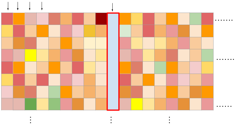
Predicting the outcome of all experiments at a new arbitrary concentration pair $(x_{1}^{*}, x_{2}^{*}) $

Predict across cell lines at a new concentration

Predicting a new output column at any unique triplet $ (c^{'},A^{'},B^{\prime})$ (a whole surface, across all concentrations).

(c1, A, B)

(c2, A, B)

(c', A, B)

(c18, A', B')

(0, 0.11)

(0,0.22)

........

(1,1)

(c', A', B')

Results

	RMSE	Pearsons's r
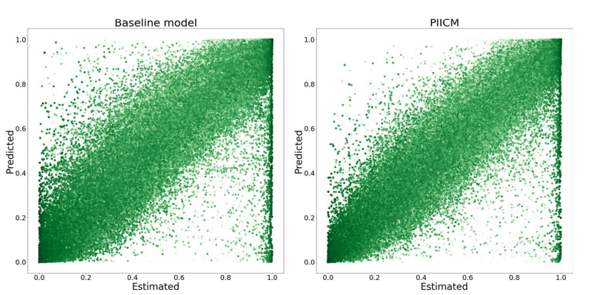
PIICM (full)	0.06802 (0.07741)	0.9882 (0.9263)
PIICM (no invariance)	0.07182 (0.07741)	0.9368 (0.9263)

Pointwise actual vs. predicted viabilities on unseen experiments.

i.e. where the triplet (c,A,B) was not a part of the training data.

Actual

() shows baseline Bliss model

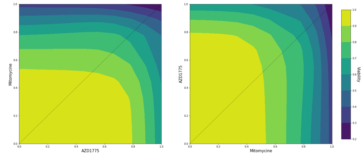
Results

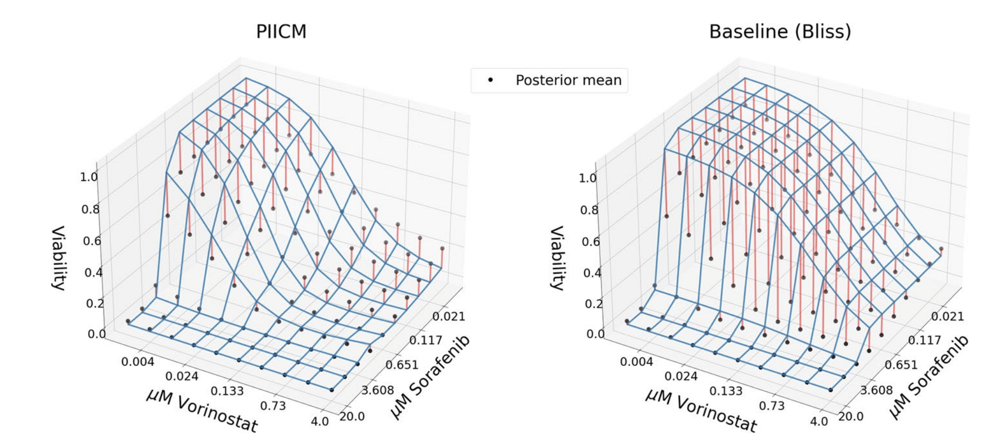
PIICM identifies drug pairs with synergestic interaction for the lung cancer cell line.

Actual viability

Predicted dose-response surface

Deviation from actual viability

RMSE

Baseline: 0.3227

PIICM: 0.1182

Future work

Currently, we cannot predict a dose-response surface for a completely unseen cell line or an unseen drug pair $ (c^{*}, A^{*}, B^{*})$ i.e. if neither $ c^{*}$ or $(A^{*}, B^{*})$ appear anywhere in the experiments.

(c1, A, B)

(c2, A, B)

(c3, A, B)

(c*, A*, B*)

Soln: Encode cell-lines with a cell embedding and encode drug pairs with a tuplet of drug embeddings.

Compute the cell kernel and drug kernel as $k_{c}(\phi(c), \phi(c^{\prime}))$ and $ k_{d}([\zeta(A), \zeta(B)], [\zeta(A^{\prime}), \zeta(B^{\prime})])$.