


Vidhi Lalchand
Postdoctoral Fellow, Broad and MIT
Vidhi Lalchand
05-04-2024
Outline
PCA
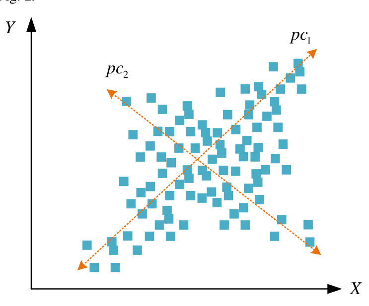
As a technique for multivariate analysis - PCA acts a foundational precursor to most unsupervised learning techniques & structure discovery.
PCA projects high-dimensional data onto the axis of maximum variance - these 'axis' or 'directions' are the eigenvectors of the covariance matrix of the data or the 'principal components.
\(y_{1}\)
\(y_{2}\)
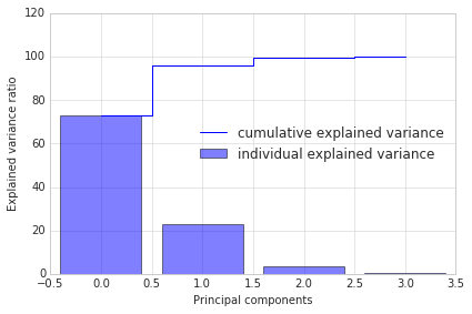
PCA workflow
The PCs are geometrically orthogonal.
Probabilistic PCA
We assume a data generation model where some high-dimensional data \(\mathbf{Y} = [\mathbf{y}_{1}....\mathbf{y}_{n}]^{T}\) are linearly related to some low-dimensional data summarised in \( \mathbf{X} \in \mathbb{R}^{N \times Q}\) and \(Q < D\).
The linear map \(\mathbf{W}\) is a \(D \times Q\) matrix and relates each \(\mathbf{x}_{n}\) to \(\mathbf{y}_{n}\), further,
The data likelihood:
Prior over latents:
Derive the marginal likelihood of the data:
(Using standard Gaussian identities as they are closed under affine operations)
Probabilistic PCA
Turns out analytical solutions exist:
Top Q eigenvectors of the sample covariance matrix \( \mathbf{S} = \dfrac{1}{N}\mathbf{Y}\mathbf{Y}^{T}\)
Diagonal matrix with Q eigenvalues
Arbitrary rotation matrix
The posterior of the latent variables can also be calculated in closed form:
(Note that regular PCA is recovered as \( \sigma^{2} \rightarrow 0\))
Probabilistic PCA ----> GPLVM
Integrate out the projection matrix \( \mathbf{W}\) and optimise the latents \(\mathbf{X}\)
Integrate out the latents \(\mathbf{X}\) and optimise the projection matrix \( \mathbf{W}\).
Method:
Method:
The linear map \(\mathbf{W}\) is a \(D \times Q\) matrix and relates each \(\mathbf{x}_{n}\) to \(\mathbf{y}_{n}\).
Prior over latents:
Prior over projection:
Basic idea: Swap what is optimised and what is integrated
(iid over rows of W)
The GPLVM methodology facilitates the use of kernels by non-linearising the map between latents \(\mathbf{X}\) and \(\mathbf{Y}\).
| Non-Probabilistic | Probabilistic (in mapping) | |
|---|---|---|
| Linear | PCA | Probabilistic-PCA |
| Non-Linear | Kernel PCA | GP-LVM |
The GPLVM is probabilistic kernel PCA with a non-linear mapping from a low-dimensional latent space \( \mathbf{X}\) to a high-dimensional data space \(\mathbf{Y}\).
Understanding the links
\(\mathbf{X}\)
Observed space
\(\mathbf{Y}\)
Given: High dimensional training data \( Y \equiv \{\bm{y}_{n}\}_{n=1}^{N}, Y \in \mathbb{R}^{N \times D}\)
Learn: Low dimensional latent space \( X \equiv \{\bm{x}_{n}\}_{n=1}^{N}, X \in \mathbb{R}^{N \times Q}\)
GPLVM Workflow
GP prior over mappings
(per dimension, \(d\))
Choice of \( \mathbf{K}\) induces non-linearity
GP marginal likelihood
Optimisation problem:
GPLVM generalises probabilistic PCA - one can recover probabilistic PCA by using a linear kernel
Feature Maps \( \rightarrow \) Kernels
A kernel \( k: \mathcal{X} \times \mathcal{X} \rightarrow \mathbb{R} \) computes an inner product in some high-dimensional embedded space where the embedding is not usually explicitly represented.
where usually, M > N.
It is also certainly possible for M to be infinite dimensional, which is the case for a Gaussian kernel. If one can reason about \( \phi \), one can derive a kernel corresponding to it by computing an inner product. This is a deterministic operation.
N x D
The Gaussian process mapping
2d latent space
High-dimensional data space
Schematic of a Gaussian process Latent Variable Model
. . .
. . .
. . .
N
D
\( Z \in \mathbb{R}^{N \times Q}\)
\( f_{d} \sim \mathcal{GP}(0,k_{\theta})\)
\( Y \in \mathbb{R}^{N \times D} (= F + noise)\)
The latents are continuous values, hence, the most popular choice of kernel function is the RBF kernel with lengthscale per dimension.
The behaviour of the lengthscales during training achieves sparsity - it prunes away redundant dimensions in the latent space.
N x D
The Gaussian process mapping
2d latent space
High-dimensional data space
Schematic of a Gaussian process Latent Variable Model
. . .
. . .
. . .
N
D
\( Z \in \mathbb{R}^{N \times Q}\)
\( f_{d} \sim \mathcal{GP}(0,k_{\theta})\)
\( Y \in \mathbb{R}^{N \times D} (= F + noise)\)
Inference modes
1. Point estimation - Learn a latent point \( \bm{x}_{n}\) per \(\bm{y}_{n}\) using the GP marginal likelihood.
2. MAP - Maximum a priori, use a prior over the latents \(p(\bm{x}_{n})\) and learn a point estimate.
3. Variational Inference with an Encoder:
GPLVM Applications: Dimensionality reduction / Clustering
Vidhi Lalchand, Aditya Ravuri, Neil D. Lawrence. Generalised GPLVM with Stochastic Variational Inference. In International Conference on Artificial Intelligence and Statistics (AISTATS), 2023
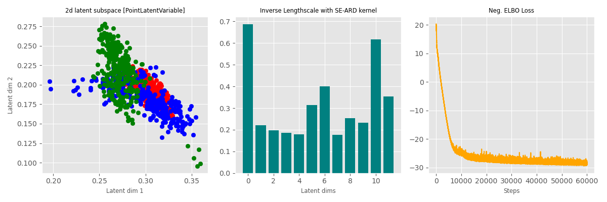
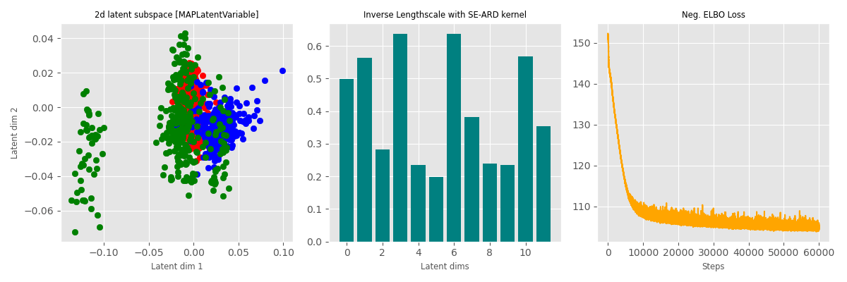
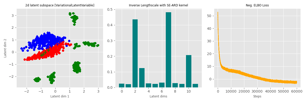
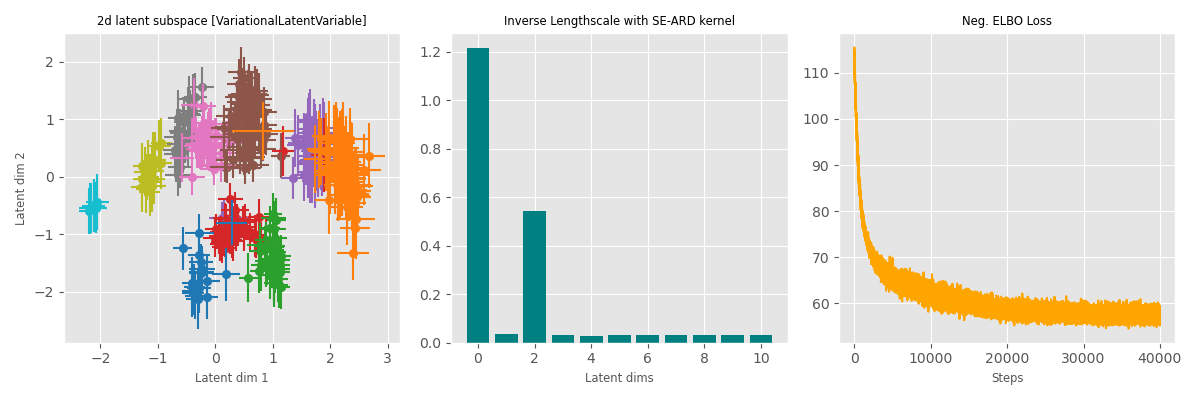
Data: Multiphase oil flow data that consists of 1000, 12 dimensional observations belonging to three known classes corresponding to different phases of oil flow.
Plot: Showing the two dimensions corresponding to the highest inverse lengthscale.
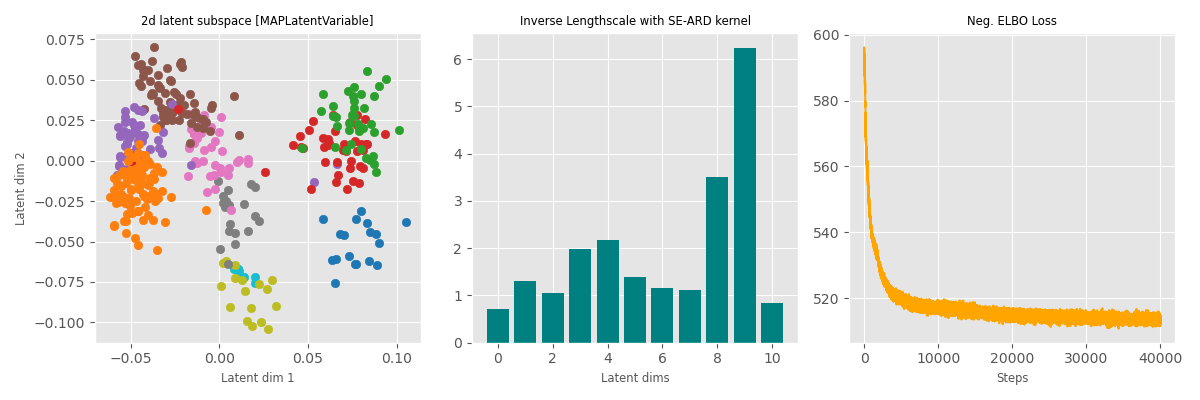
The probabilistic method (which learn a latent distribution per data point, 3rd row) switches off 7 out of 10 latent dimensions - the point estimation methods are not able to achieve that pruning.
Point estimate
MAP (point est. with a prior)
Bayesian (Variational Inference)
Dominant dimensions
Inv. Lengthscale per dim.
ELBO Loss
GPLVM Applications: Dimensionality reduction / Clustering
Vidhi Lalchand, Aditya Ravuri, Neil D. Lawrence. Generalised GPLVM with Stochastic Variational Inference. In International Conference on Artificial Intelligence and Statistics (AISTATS), 2023
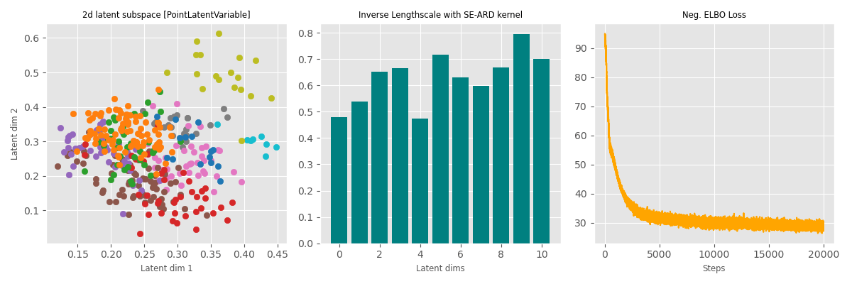
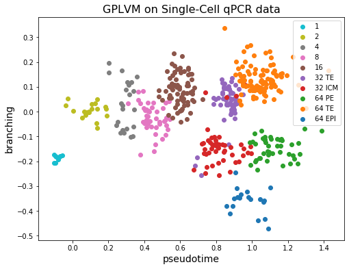
Data: qPCR data for 48 genes obtained from mice. The data contains 48 columns, with each column corresponding to (normalized) measurements of each gene. Cells differentiate during their development and these data were obtained at various stages of development. The various stages are labelled from the 1-cell stage to the 64-cell stage.
Point estimate
MAP (point est. with a prior)
Bayesian
Dominant dimensions
Inv. Lengthscale per dim.
ELBO Loss
Benchmark reconstruction
For the 32-cell stage, the data is further differentiated into ‘trophectoderm’ (TE) and ‘inner cell mass’ (ICM). ICM further differentiates into ‘epiblast’ (EPI) and ‘primitive endoderm’ (PE) at the 64-cell stage.
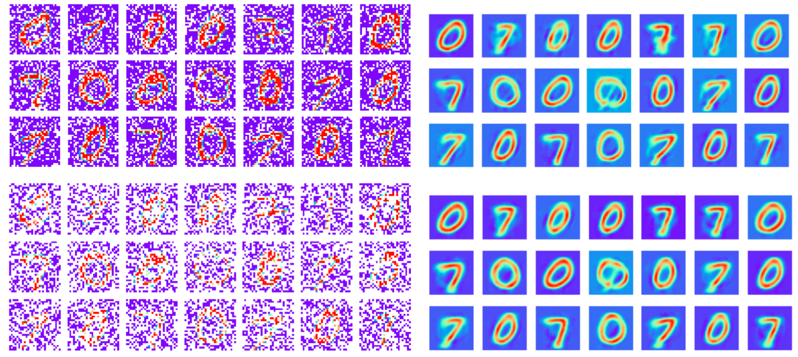
GPLVM Applications: Learning from partially complete / masked data
30%
60%
Training data: MNIST images with masked pixels
Reconstruction
The model achieves disentanglement in the two dominant latent dimensions
Note: This is different to tasks where missing data is only introduced at test time
Trained with ~40% missing pixels
Vidhi Lalchand, Aditya Ravuri, Neil D. Lawrence. Generalised GPLVM with Stochastic Variational Inference. In International Conference on Artificial Intelligence and Statistics (AISTATS), 2023
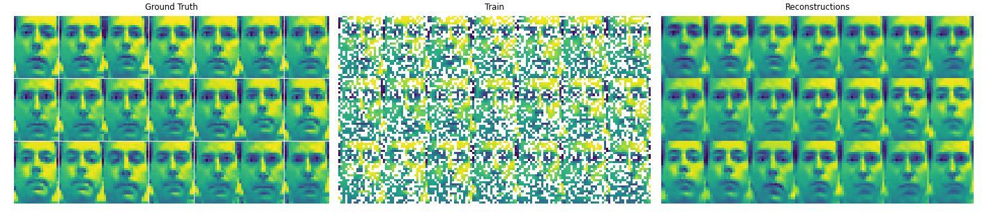
Data: Frey Faces taken from a taken from a video sequence that consists of 1965 images of size 28×20.
GPLVM Applications: Learning from partially complete / masked data
Ground truth
Test data
Reconstruction
Vidhi Lalchand, Aditya Ravuri, Neil D. Lawrence. Generalised GPLVM with Stochastic Variational Inference. In International Conference on Artificial Intelligence and Statistics (AISTATS), 2023
GPLVM Applications: Learning dynamical data
Summary
Thank you!
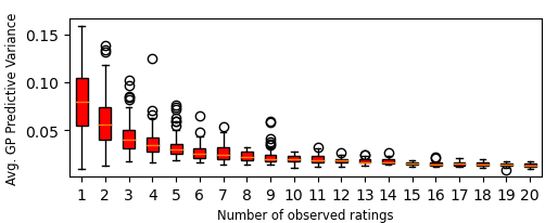
Learning from massively missing data: Movie ratings
Method | PMF | BiasMF | NNMF | GPLVM
MovieLens100K | 0.952 | 0.911 | 0.903 | 0.924
Test reconstruction accuracy
Interpretable uncertainty: The confidence in predictions is higher when there is more data about a user.
Data: 943 users, 1638 movies (avg user has rated approx 20 movies)
By Vidhi Lalchand


