Vidhi Lalchand
Postdoctoral Fellow, Broad and MIT
Vidhi Lalchand
Wessel P. Bruinsma
David R. Burt
Carl E. Rasmussen
Motivation
Mathematical set-up
Inputs
Outputs
Latent function prior
Factorised Gaussian likelihood
Inducing locations
Inducing variables
"Collapsed ELBO"
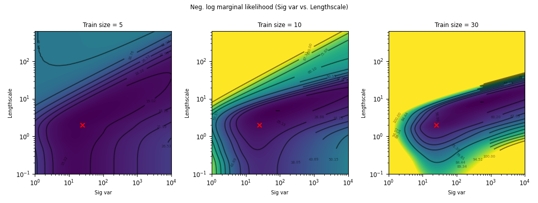
Hyperparameter inference
Michalis Titsias. Variational learning of inducing variables in sparse Gaussian processes. In Artificial intelligence and statistics, pages 567-574. PMLR, 2009.
intelligence and statistics, pages 567–574. PMLR, 2009
Titsias [2009] showed that in the case of a Gaussian likelihood the optimal variational distribution \( q^{*}(u)\) is Gaussian and can be derived in closed-form.
Canonical Inference for \( \theta\) in sparse GPs:
Variational approximation to the posterior
[Ours] Doubly collapsed Inference for \( \theta\) in sparse GPs:
Hyperparameter inference
Variational approximation to the posterior
"Collapsed ELBO"
Algorithm
Overall, the core training algorithm alternates between two steps:
By sampling from \( q^{*}(\bm{\theta})\), we side-step the need to sample from the joint \( (\bm{u},\bm{\theta})\)-space yielding a significantly more efficient algorithm in the case of regression with a Gaussian likelihood.
James Hensman, Alexander G Matthews, Maurizio Filippone, and Zoubin Ghahramani. MCMC for variationally Sparse Gaussian processes. In Advances in Neural Information Porcessing Systems, pages 1648-1656, 2015.
pages 1648–1656, 2015bintelligence and statistics, pages 567–574. PMLR, 2009
\( n_{\theta}\) is the number of hyperparameters and \(m\) is the number of inducing variables
\( \log p(\bm{y}) \geq \int q(\bm{\theta}) \mathcal{L}_{\bm{\theta}, Z}d\bm{\theta} - \textrm{KL}(q(\bm{\theta}) || p(\bm{\theta})) \)
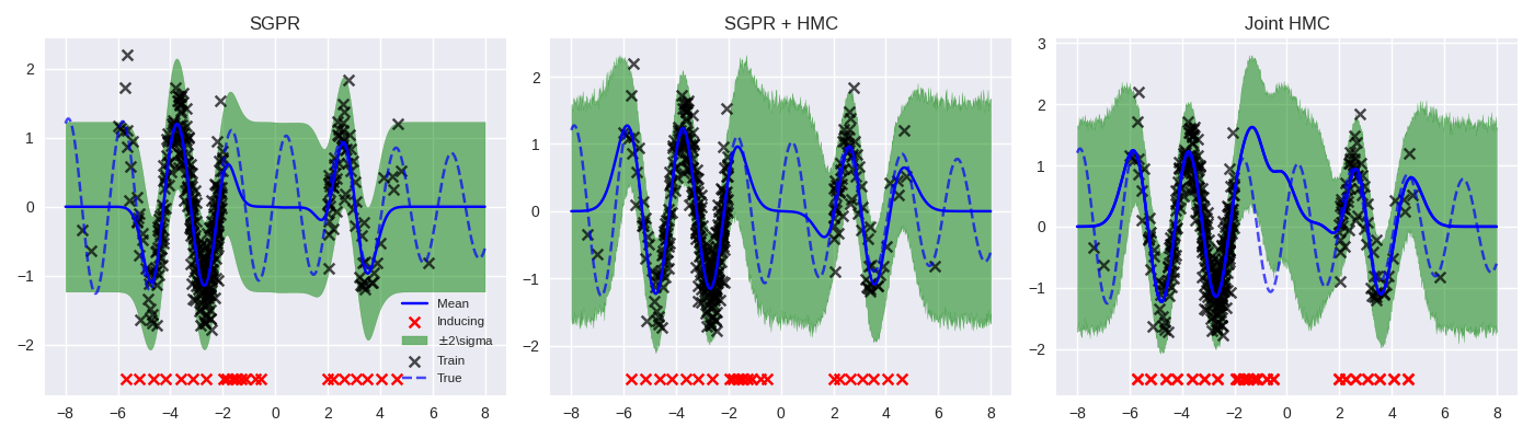
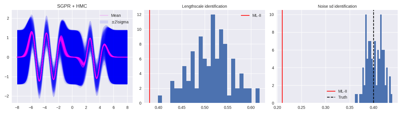
1d Synthetic Experiment
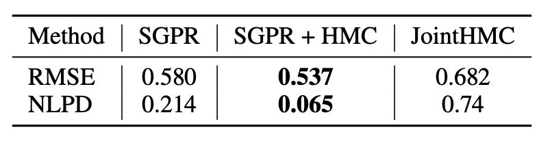
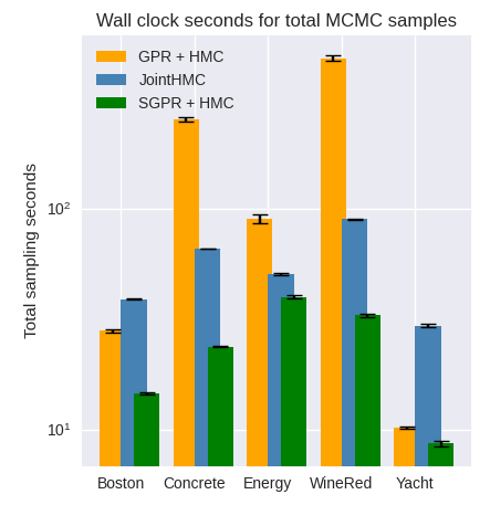
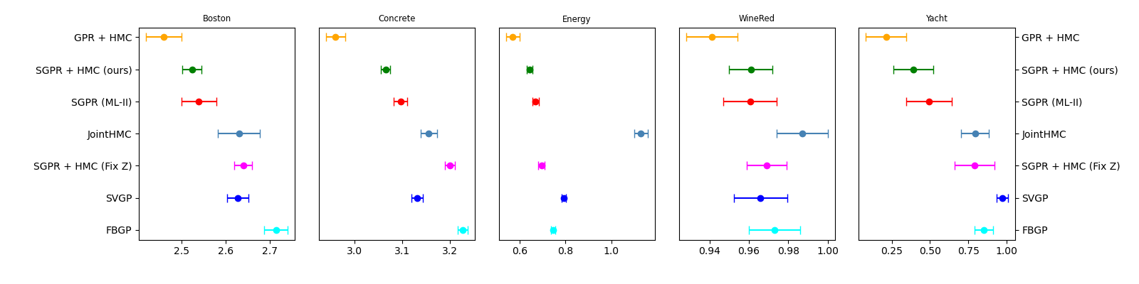
Sparse GP Benchmarks
Neg. log predictive density (mean \(\pm\) se) on test data, 10 splits.
Thank you!
By Vidhi Lalchand


