


Vidhi Lalchand
Postdoctoral Fellow, Broad and MIT
Vidhi Lalchand
Research Highlights
13-02-2025
(A compilation of research directions over the last few years and a snapshot of current research)
Outline
- Thomas Garrity
Gaussian processes are a Bayesian nonparametric paradigm for learning "functions".
Gaussian Processes
Gaussian Processes: A generalisation of a Gaussian distribution
A sample from a \(k\)-dimensional Gaussian \( \mathbf{x} \sim \mathcal{N}(\mu, \Sigma) \) is a vector of size \(k\). $$ \mathbf{x} = [x_{1}, \ldots, x_{k}] $$
A GP is an infinite dimensional analogue of a Gaussian distribution (so samples are functions \( \Leftrightarrow \)vectors of infinite length)
The mathematical crux of a GP is that \( \textbf{f} \equiv [f(x_{1}), f(x_{2}), f(x_{3}),....., f(x_{N})]\) is just a draw from a N-dimensional multivariate Gaussian.
But at any given point, we only need to represent our function \( f(x) \) at a finite index set \( \mathcal{I} = [x_{1},\ldots, x_{500}]\). So we are interested in our 500 dimensional function vector \( [f(x_{1}), f(x_{2}), f(x_{3}),....., f(x_{500})]\).
Marginalising function values corresponding to inputs not in our index set.
Gaussian processes
A powerful, Bayesian, non-parametric paradigm for learning functions.
\(f(x) \sim \mathcal{GP}(m(x), k_{\theta}(x,x^{\prime})) \)
\(f(X) \sim \mathcal{N}(m(X), K_{X})\)
For a finite set of points, \( X \):
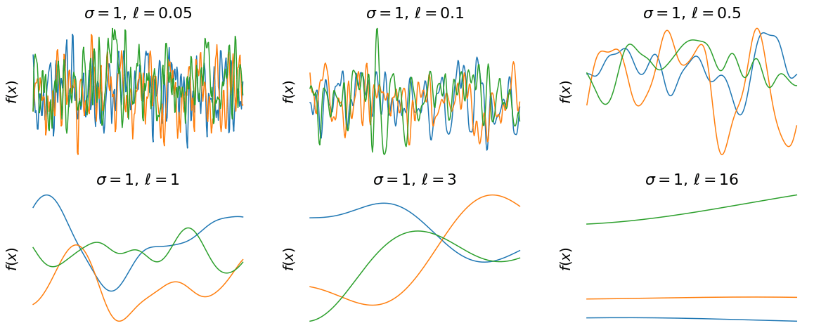
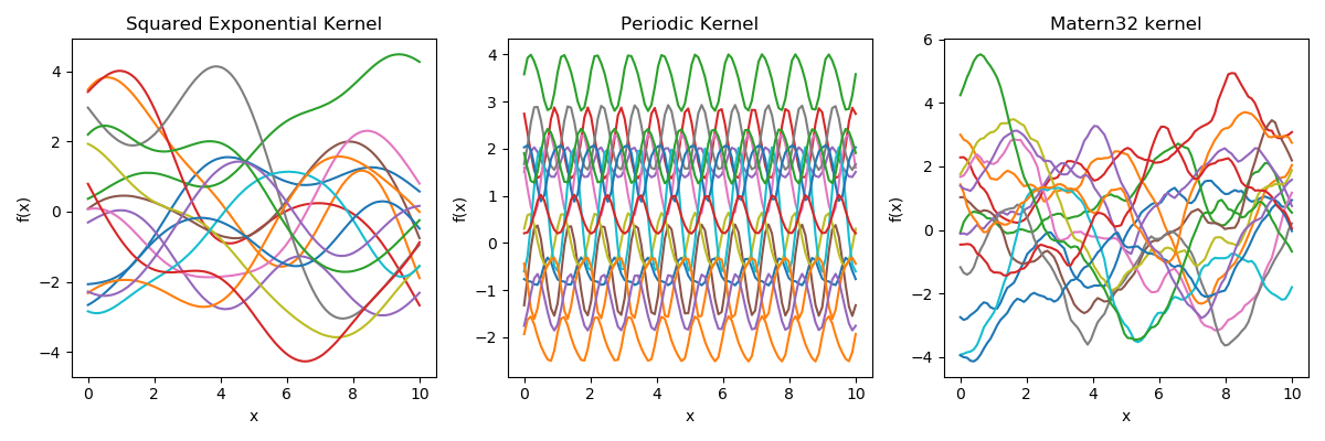
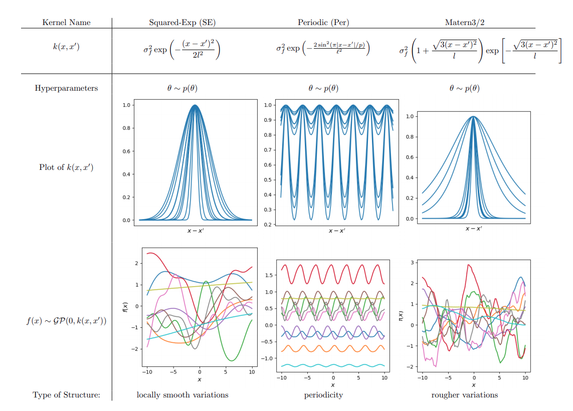
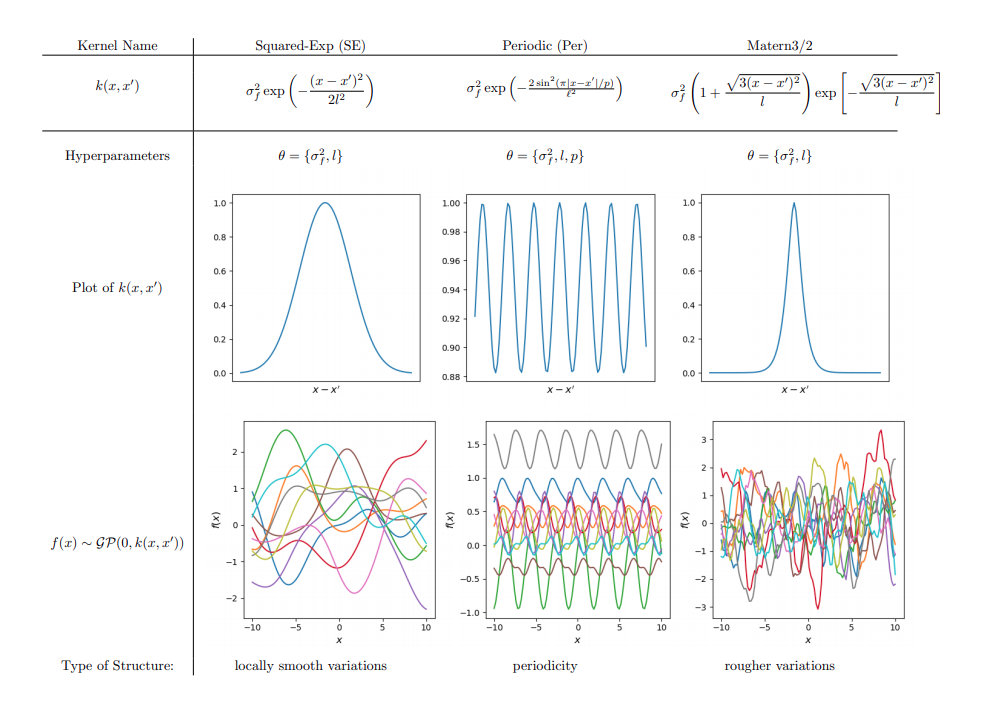
\( k_{\theta}(x,x^{\prime})\) encodes the support and inductive biases in function space.
GP Math: Canonical GPs
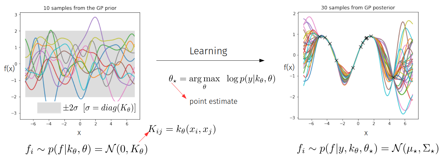
Learning occurs through adapting the hyperparameters of the kernel function by optimising the marginal likelihood.
A central quantity in Bayesian ML is the marginal likelihood.
Learning Step:
Data likelihood
Prior
Denominator of Bayes Rule
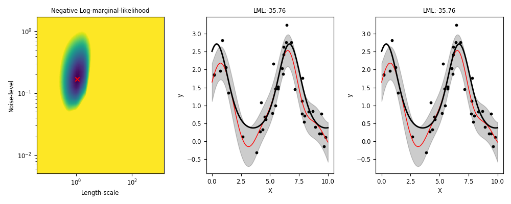
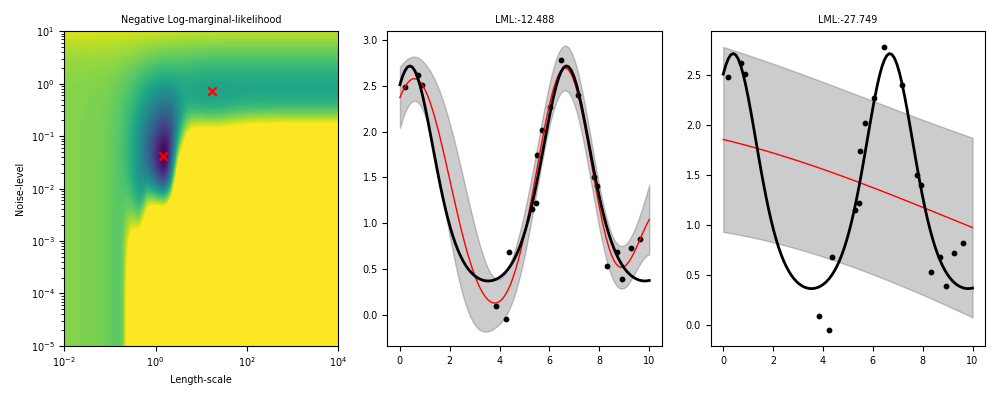
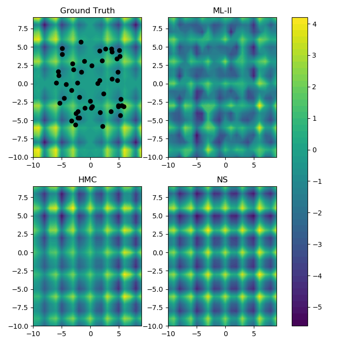
Behaviour of ML-II
Non-identifiability of ML-II under weak data, multiple restarts needed.
ML-II - does it always work?
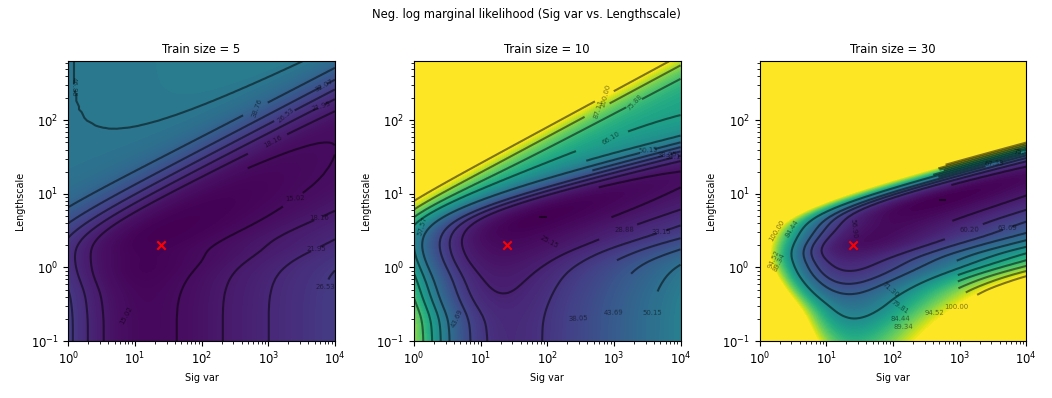
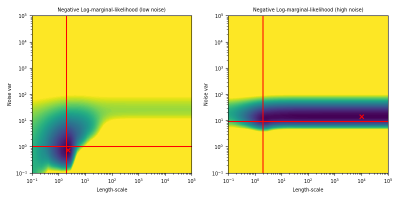
Weakly identified hyperparameters can manifest in flat ridges (where different combinations of hyperparameters give very similar ML values) in the marginal likelihood surface, making ML-II estimates subject to high-variability.
The problem of ridges in the marginal likelihood surface also does not necessarily go away as more observations are collected.
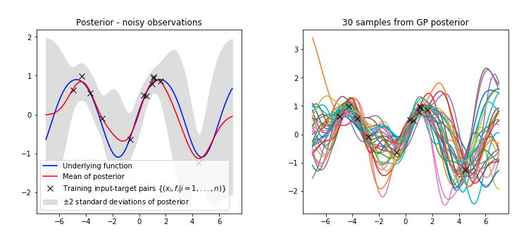
A fully Bayesian treatment of GP models would integrate away kernel hyperparameters when making predictions:
where \( \bm{f}_{*}| X_{*}, X, \bm{y}, \bm{\theta} \sim \mathcal{N}(\bm{\mu_{*},\Sigma_{*}}) \)
The posterior over hyperparameters is given by,
where \(p(\bm{y}|\bm{\theta}) \) is the GP marginal likelihood.
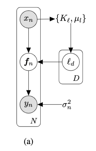
Hierarchical GPs
Propagate hyperparameter uncertainty to outputs.
Hyperprior \( \rightarrow \)
Prior \( \rightarrow \)
Model \( \rightarrow \)
Likelihood \( \rightarrow \)
Intractable
Integrating out kernel hyperparameters gives rise to an approximate posterior which is a heavy-tailed non-Gaussian process, this may make it a better choice for certain applications.
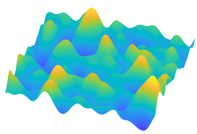
Visualising the prior predictive function space
Canonical
Hierarchical
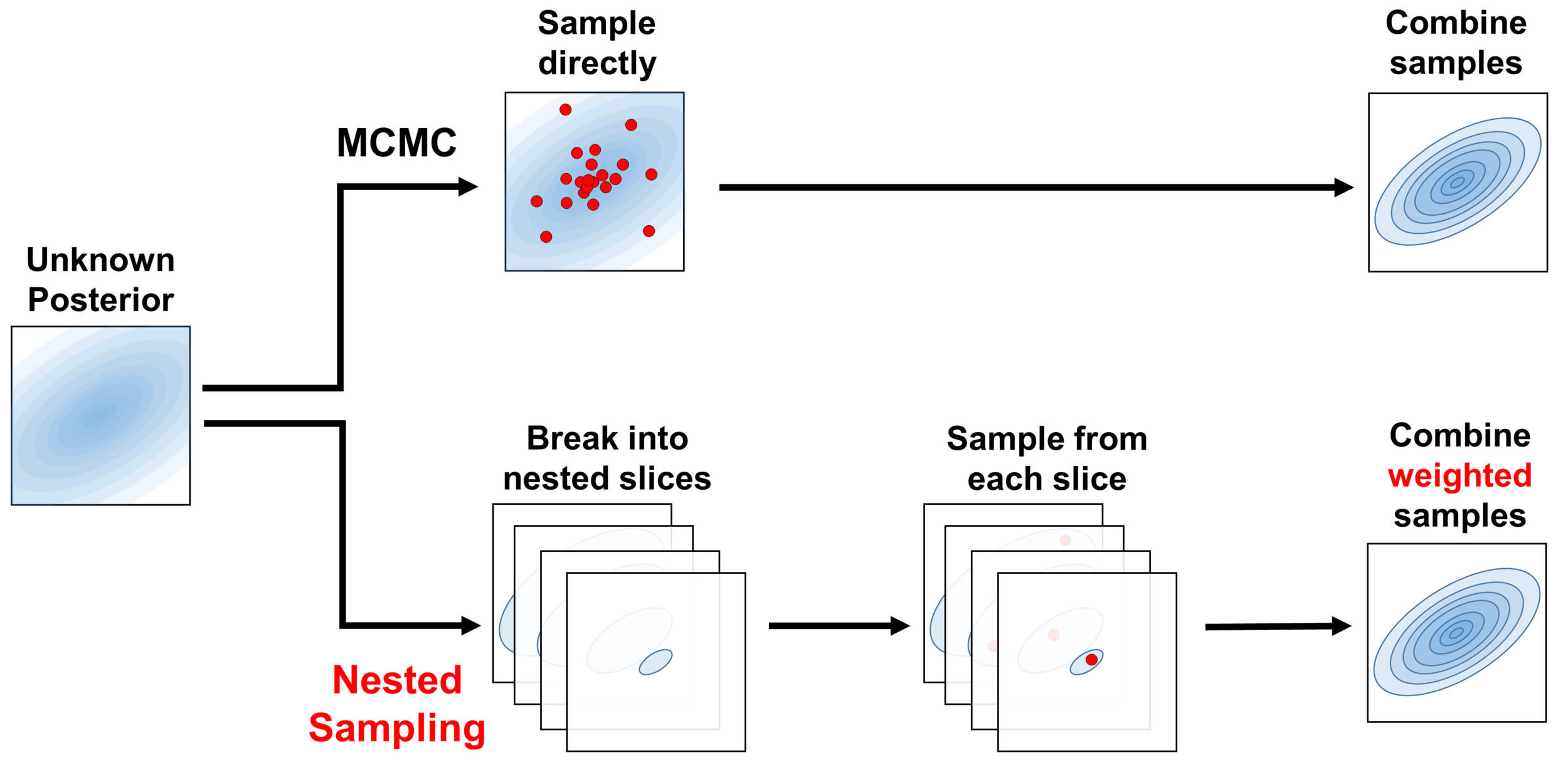
We adapt a technique frequently used in physics and astronomy literature to sample from the hyperparameter posterior.
Nested Sampling (Skilling, 2004) is a gradient free method for Bayesian computation.
Fergus Simpson*, Vidhi Lalchand*, Carl E. Rasmussen. Marginalised Gaussian processes with Nested Sampling . https://arxiv.org/pdf/2010.16344.pdf
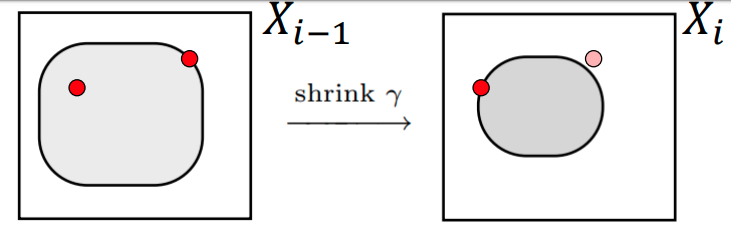
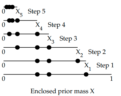
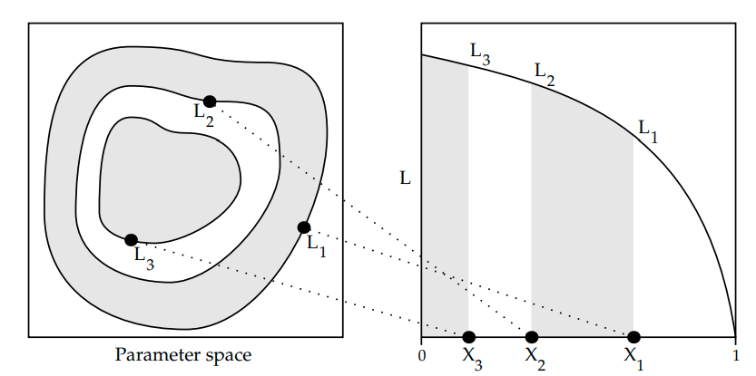
Principle: Sample from "nested shells" / iso-likelihood contours of the evidence and weight them appropriately to give posterior samples.
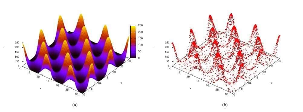
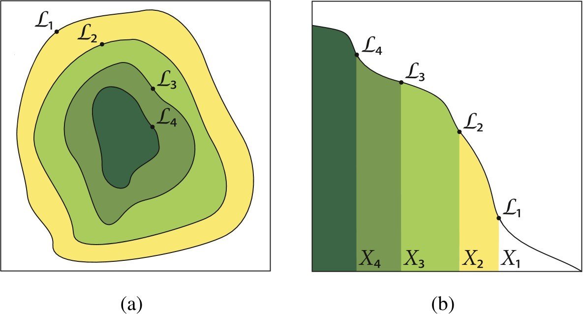
Nested Sampling: The principle
Sample a new point \( \theta^{\prime}\) from the prior subject to \( \mathcal{L}(\theta^{\prime}) > \mathcal{L}_{i} \)
Define a notion of prior volume, $$ X(\lambda) = \int_{\mathcal{L}(\theta) > \lambda} \pi(\theta)d\theta$$
The area/volume of parameter space "inside" a iso-likelihood contour
One can re-cast the multi-dimensional evidence integral as a 1d function of prior volume \( X\).
$$ \mathcal{Z} = \int \mathcal{L}(\theta)\pi(\theta)d\theta = \int_{0}^{1} \mathcal{L}(X)dX$$
$$ \mathcal{Z} \approx \sum_{i=1}^{M}\mathcal{L_{i}}(X_{i} - X_{i+1})$$
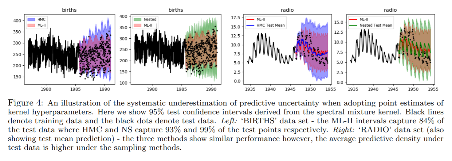
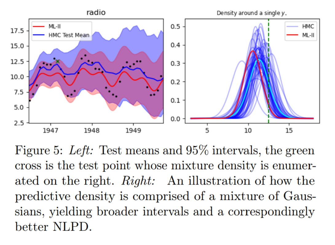
Results
Why does a more diffused predictive interval yield better test predictive density?
Fergus Simpson*, Vidhi Lalchand*, Carl E. Rasmussen. Marginalised Gaussian processes with Nested Sampling . https://arxiv.org/pdf/2010.16344.pdf
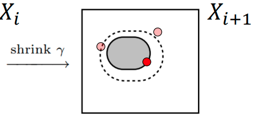
2d modelling task
Time series data: ML-II v. HMC v. Nested
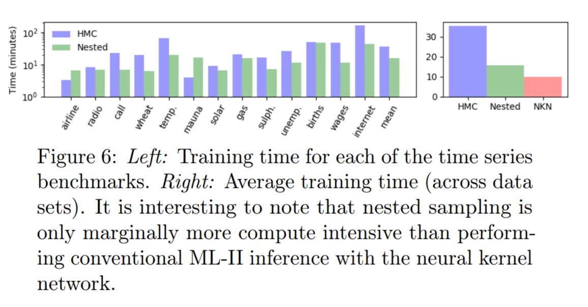
HMC v. Nested (Training runtime)
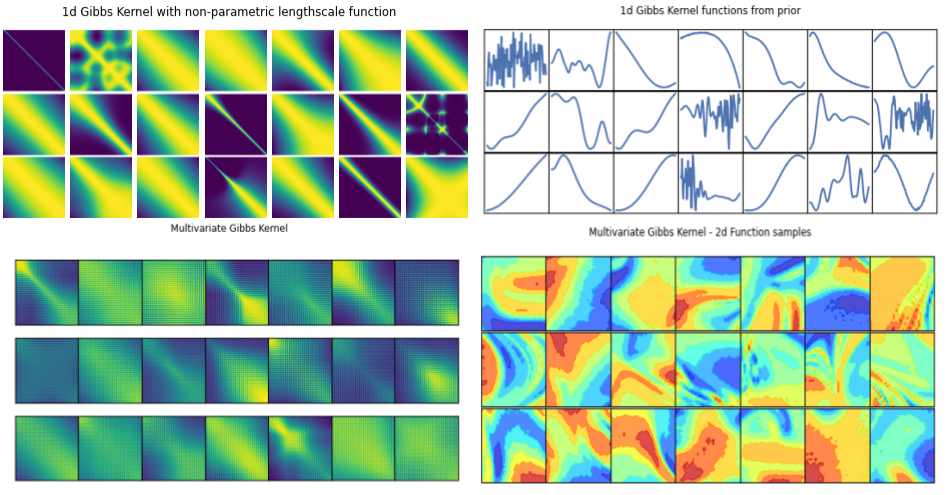
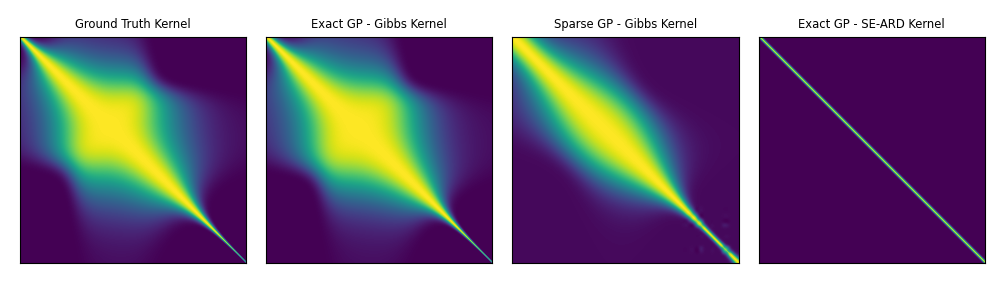
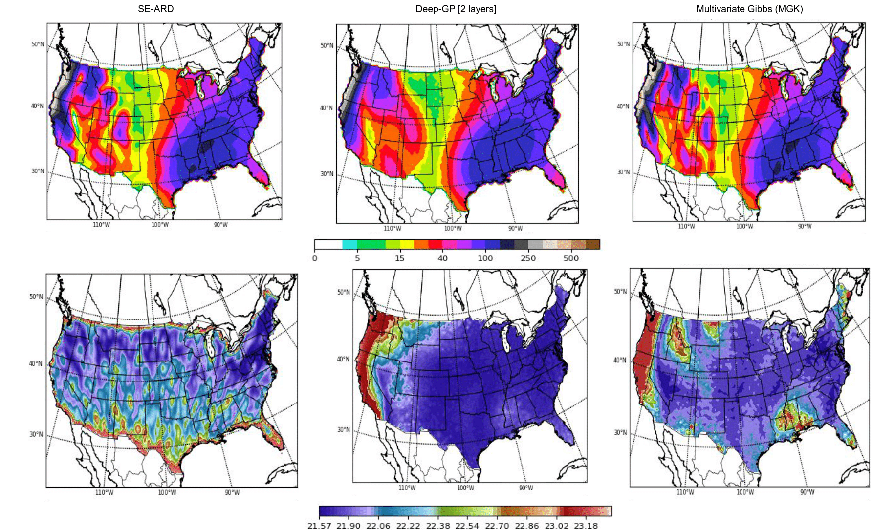
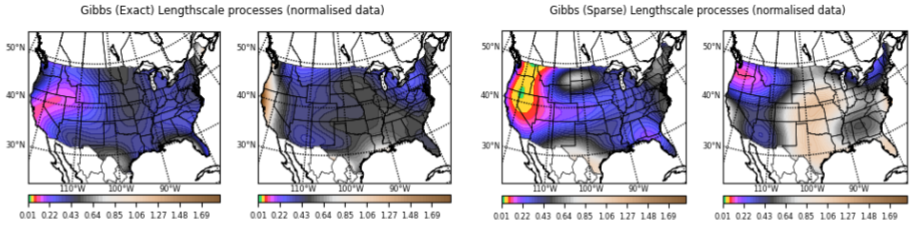
Gibbs kernel:
Hierarchical Non-stationary Gaussian Processes: Gibbs Kernel
Stationary kernels assume fixed inductive biases across the whole input space, where the smoothness and structure properties do not change over the space of covariates/inputs.
Non-stationary kernels allow hyperparameters to be input-dependent, in a hierarchical setting, these functions can in turn be modelled probabilistically.
Prior Predictive samples
Hierarchical GP Model: MAP Inference
Classical
Stationary Hierarchical
Non-Stationary Hierarchical
Hyperprior \( \rightarrow \)
Prior \( \rightarrow \)
Model \( \rightarrow \)
Likelihood \( \rightarrow \)
Hyperprior \( \rightarrow \)
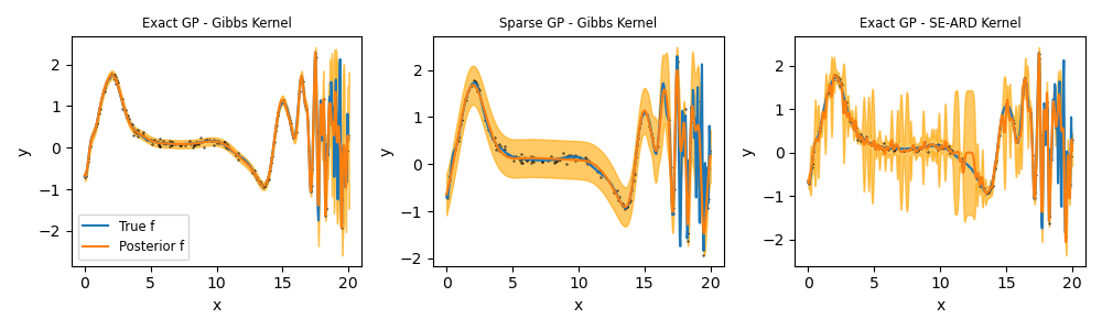
Synthetic Examples: 1d and 2d
Exact GP - SE-ARD
Exact GP - Gibbs Kernel
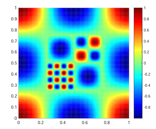
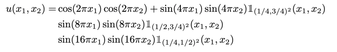
Ground truth function surface
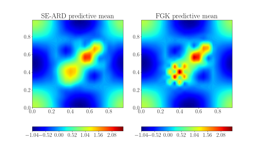
Posterior predictive means
Kernel matrix post training
Kernel matrix with ground truth hyperparameters
Learning a truncated trigonometric function in 2d
Stationary kernel
Means
Variances
Non-stationary
Lengthscale processes across the input space
Modelling Precipitation across the US
Source: National Oceanic Atmospheric Administration (https://www.ncei.noaa.gov/cdo-web/)
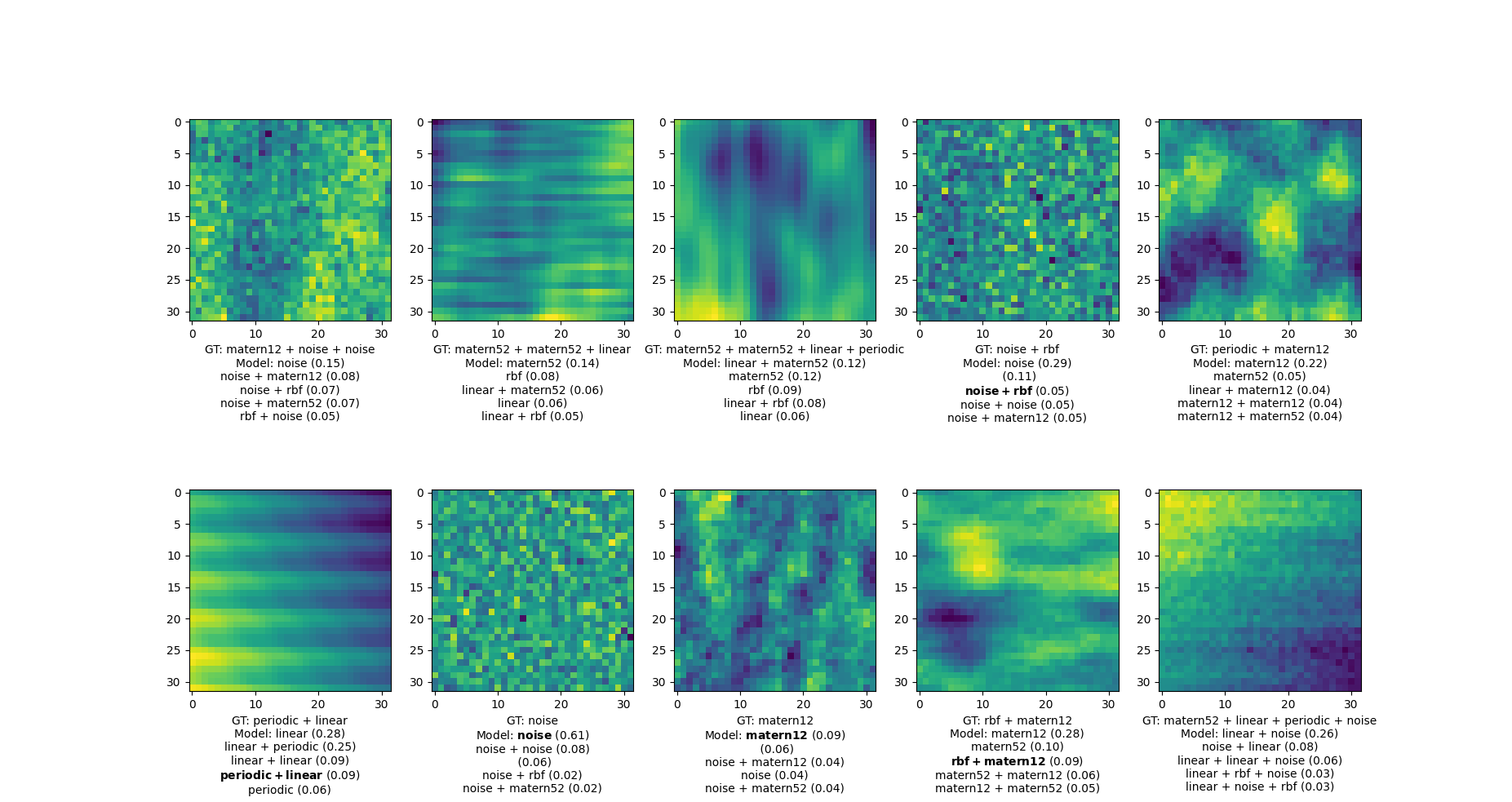
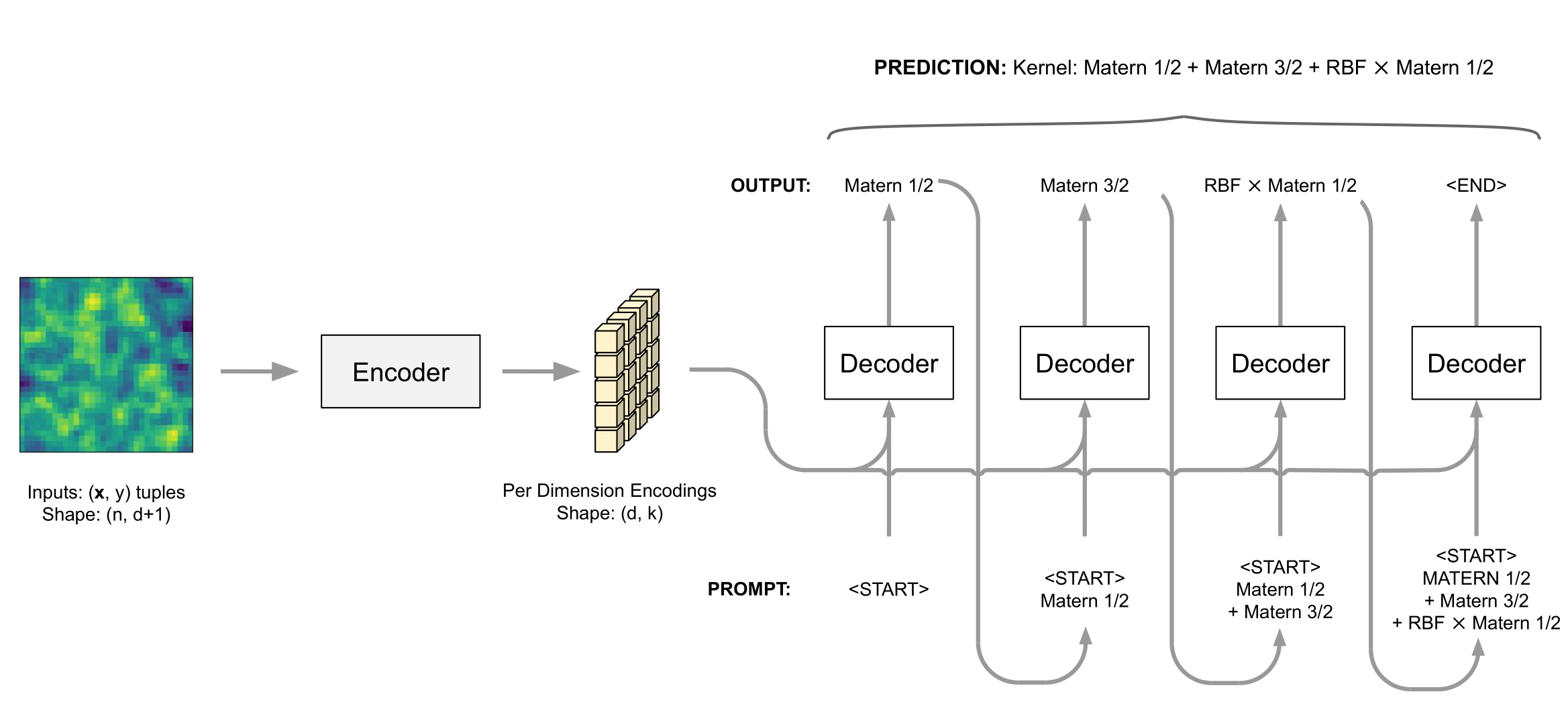
Kernel Identification with Transformers
A framework for performing kernel selection via a transformer deep neural network.
(a) The ability to identify multiple candidate kernels compatible with the data.
(b) It is blazingly fast to evaluate once it is pre-trained
Training data
Labels: RBF*PER + MAT52
+
Transformer DNN
RBF {0.43}
MAT52 {0.31}
RBF + NOISE {0.2}
RBF + MAT52 {0.06}
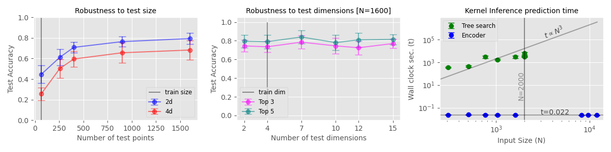
Kernel Identification with Transformers
Kernel Identification with Transformers
Left: Classification performance for random samples drawn from primitive kernels across a range of test sizes and dimensionality.
Right: The time taken to predict a kernel for each of the UCI datasets. While KITT's overhead remains approximately constant, the tree search becomes impractical for larger inputs.
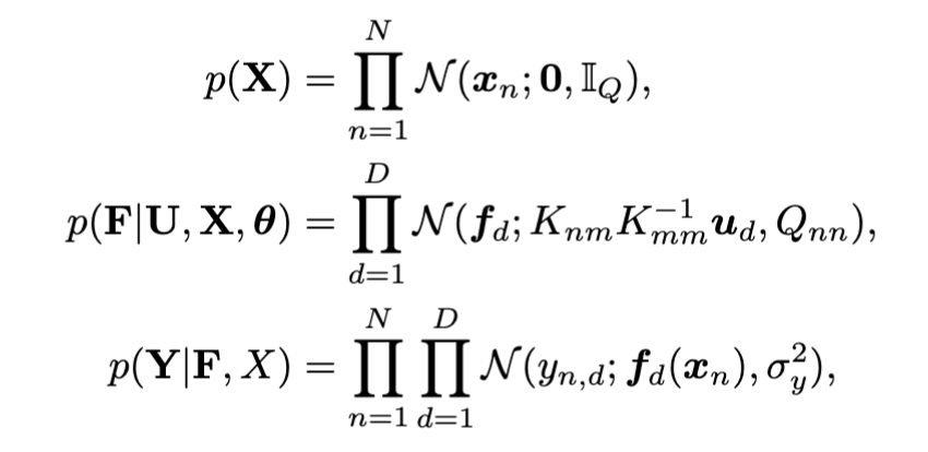
Given: High dimensional training data \( \mathbf{Y} \equiv \{\bm{y}_{n}\}_{n=1}^{N}, Y \in \mathbb{R}^{N \times D}\)
Learn: Low dimensional latent space \( \mathbf{X} \equiv \{\bm{x}_{n}\}_{n=1}^{N}, X \in \mathbb{R}^{N \times Q}\)
Lalchand et al. (2022)
Gaussian Processes for Latent Variable Modelling (at scale)
Vidhi Lalchand, Aditya Ravuri, Neil D. Lawrence. Generalised GPLVM with Stochastic Variational Inference. In International Conference on Artificial Intelligence and Statistics
(AISTATS), 2022
The GPLVM is probabilistic kernel PCA with a non-linear mapping from a low-dimensional latent space \( \mathbf{X}\) to a high-dimensional data space \(\mathbf{Y}\).
The Gaussian process mapping
High-dimensional data space
. . .
. . .
N
D
\( X \in \mathbb{R}^{N \times Q}\)
\( f_{d} \sim \mathcal{GP}(0,k_{\theta})\)
\( Y \in \mathbb{R}^{N \times D} (= F + noise)\)
GP prior over mappings
(per dimension, \(d\))
GP marginal likelihood
Optimisation problem:
GPLVM generalises probabilistic PCA - one can recover probabilistic PCA by using a linear kernel
Gaussian Processes for Latent Variable Modelling (at scale)
Lalchand et al. (2022)
. . .
N
D
\( \mathbf{X} \in \mathbb{R}^{N \times Q}\)
\( f_{d} \sim \mathcal{GP}(0,k_{\theta})\)
\( \mathbf{Y} \in \mathbb{R}^{N \times D} (= F + noise)\)
ELBO:
Stochastic Variational Formulation
prohibitive
Prior on latents
Prior on inducing variables
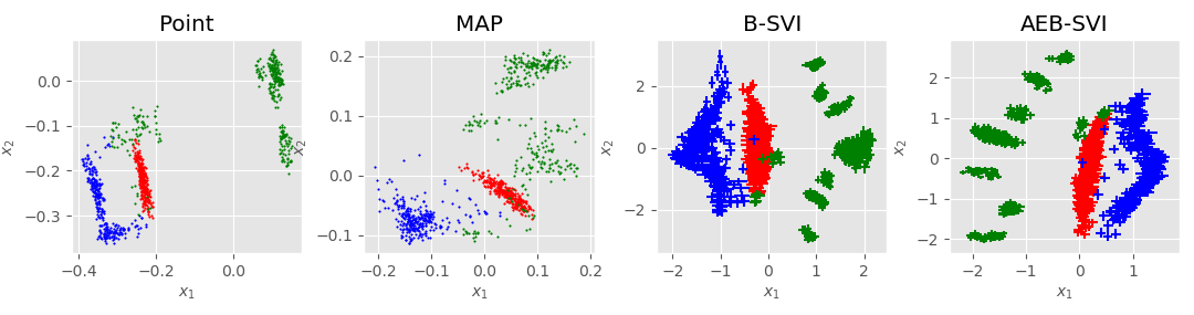
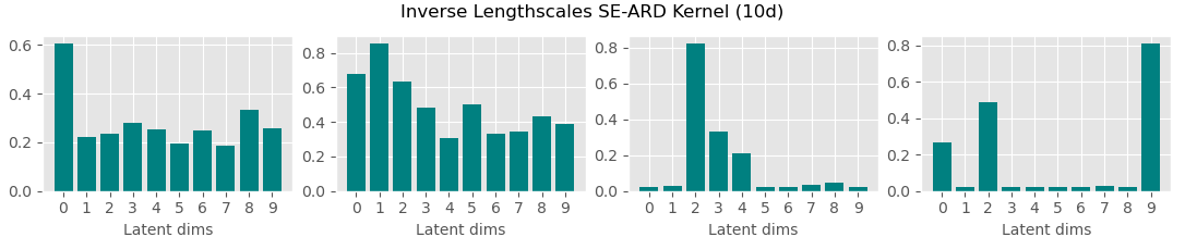
Bayesian GPLVM: Automatic relevance determination (ARD)
Vidhi Lalchand, Aditya Ravuri, Neil D. Lawrence. Generalised GPLVM with Stochastic Variational Inference. In International Conference on Artificial Intelligence and Statistics
(AISTATS), 2022
In the plot: Showing the two dimensions corresponding to the highest inverse lengthscale.
In the plot: Inverse lengthscales for each latent dimension. Both modes of inference switch off 7 out of 10 dimensions.
Data: Multiphase oil flow data that consists of 1000, 12 dimensional observations belonging to three known classes corresponding to different phases of oil flow.
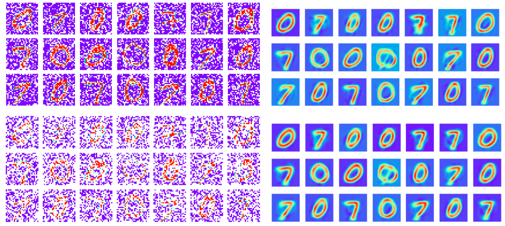
Decoder only
Encoder-Decoder
GPLVMs are typically decoder only models but can be amortised with an encoder network to learn parameters of the variational distribution
Robust to missing dimensions in training data (missing at random)
Vidhi Lalchand, Aditya Ravuri, Neil D. Lawrence. Generalised GPLVM with Stochastic Variational Inference. In International Conference on Artificial Intelligence and Statistics
(AISTATS), 2022
30%
60%
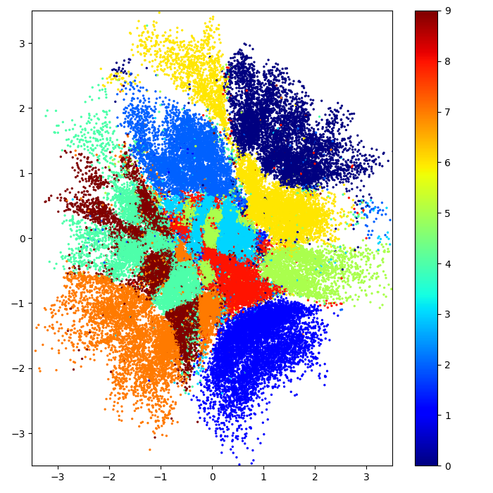
Training data: MNIST images with masked pixels
Reconstruction
Note: This is different to tasks where missing data is only introduced at test time
Learning to reconstruct dynamical data
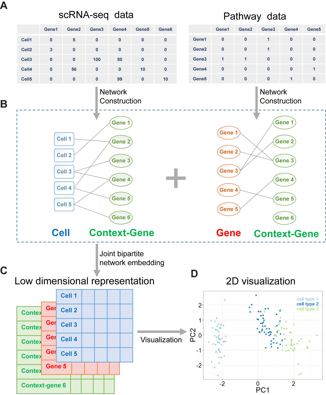
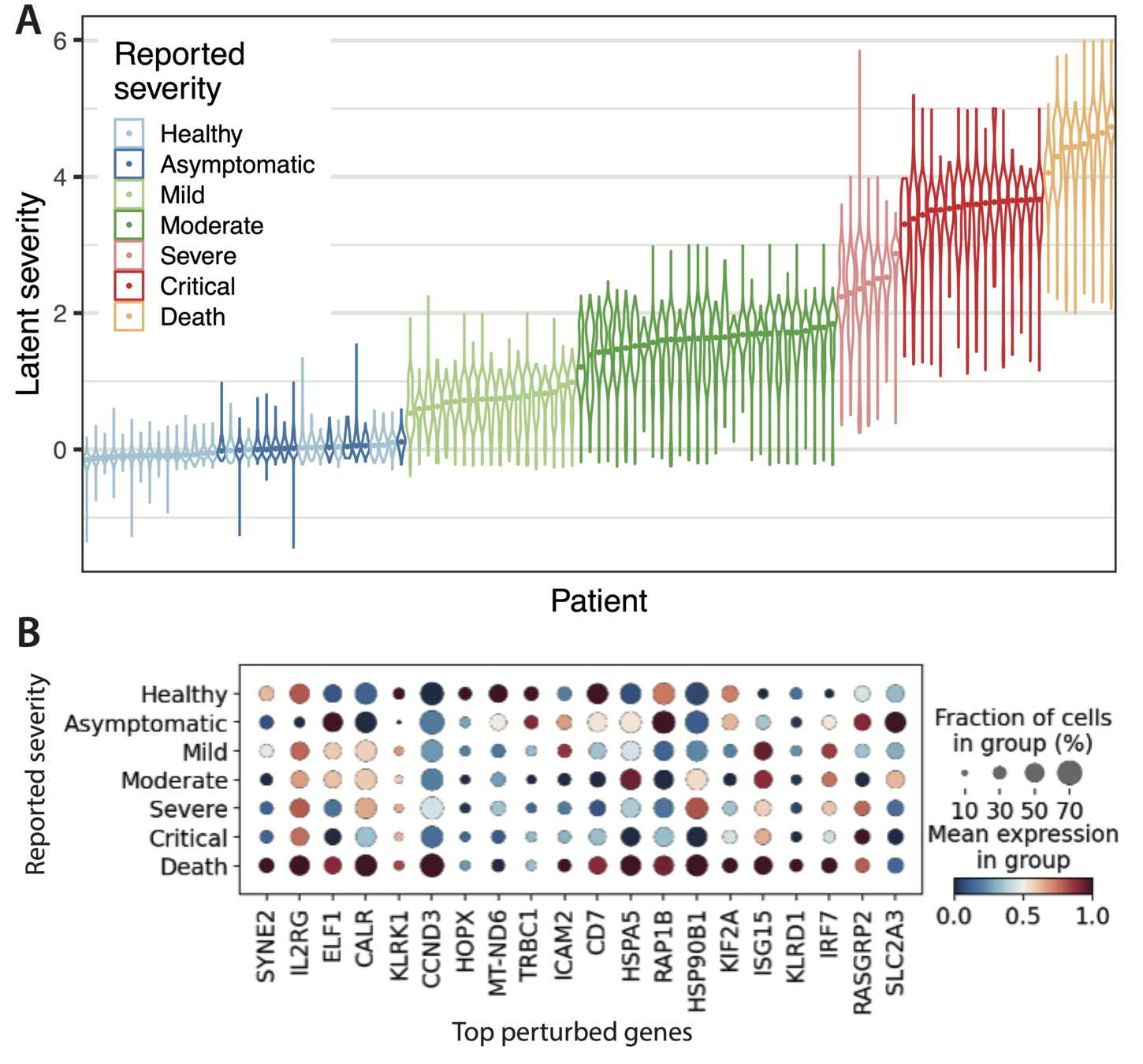
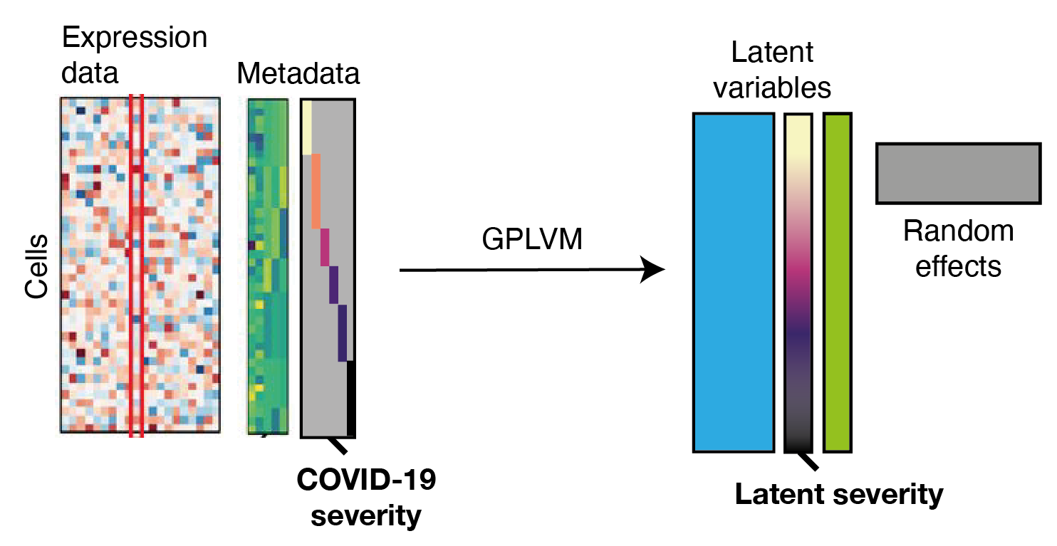
Learning interpretable latent dimensions in biological data
Vidhi Lalchand*, Aditya Ravuri*, Emma Dann*, Natsuhiko Kumasaka, Dinithi Sumanaweera, Rik G.H. Lindeboom, Shaista Madad, Neil D. Lawrence, Sarah A. Teichmann. Modelling Technical and Biological Effects in single-cell RNA-seq data with Scalable Gaussian Process Latent Variable Models (GPLVM). In Machine Learning in Computational Biology (MLCB), 2022
COVID Data: Gene expression profiles of peripheral blood mononuclear cells (PBMC) from a cohort of 107 patients.
N = 600,000 cells
Data dimension D = 5000
Latent dimension Q = 10
One of the latent dimensions captures gradations of COVID severity across patients. when averaged
The model is able to find structure in the gene expression profile
In the plot: Schematic of the GPLM model learning a mapping from a low-dimensional latent space to gene expression profiles per cell.
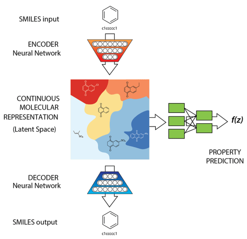
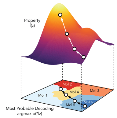
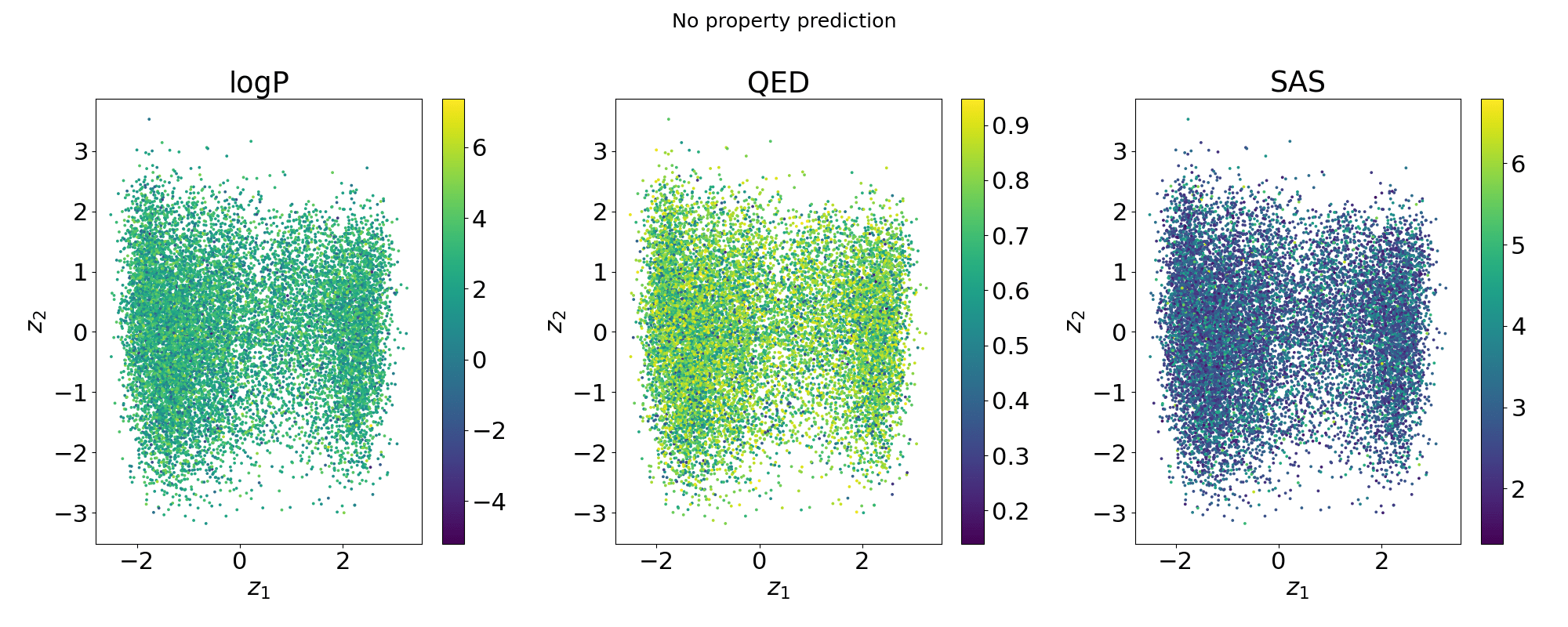
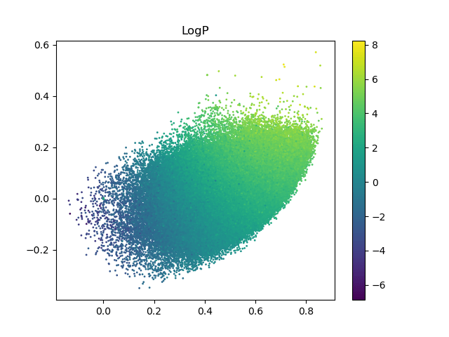
Generative model for small molecules + Property prediction
How do we use generative modelling to identify molecules which optimise a property of interest?
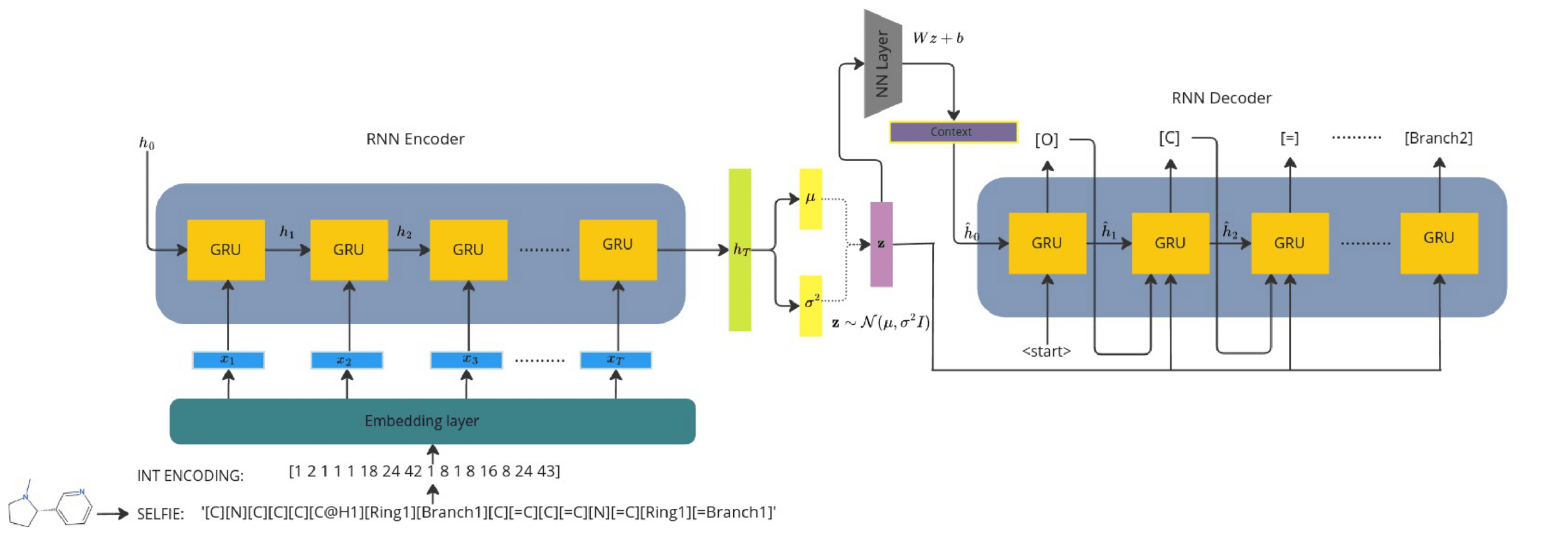
Gómez-Bombarelli R, et al. Automatic chemical design using a data-driven continuous representation of molecules. ACS central science. 2018. (ChemicalVAE)
Generative model for small molecules + Property prediction
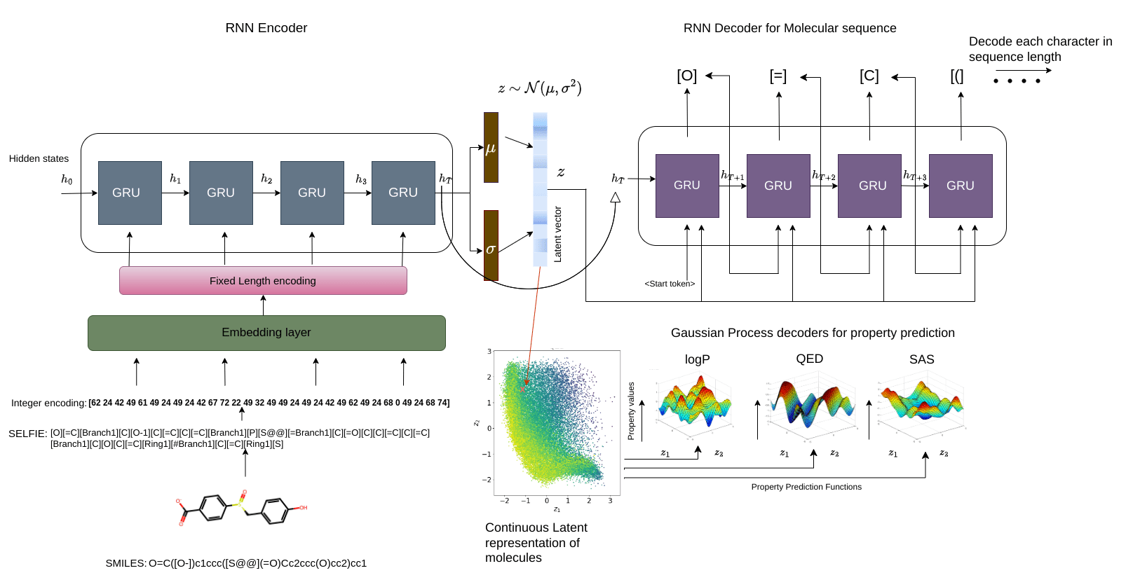
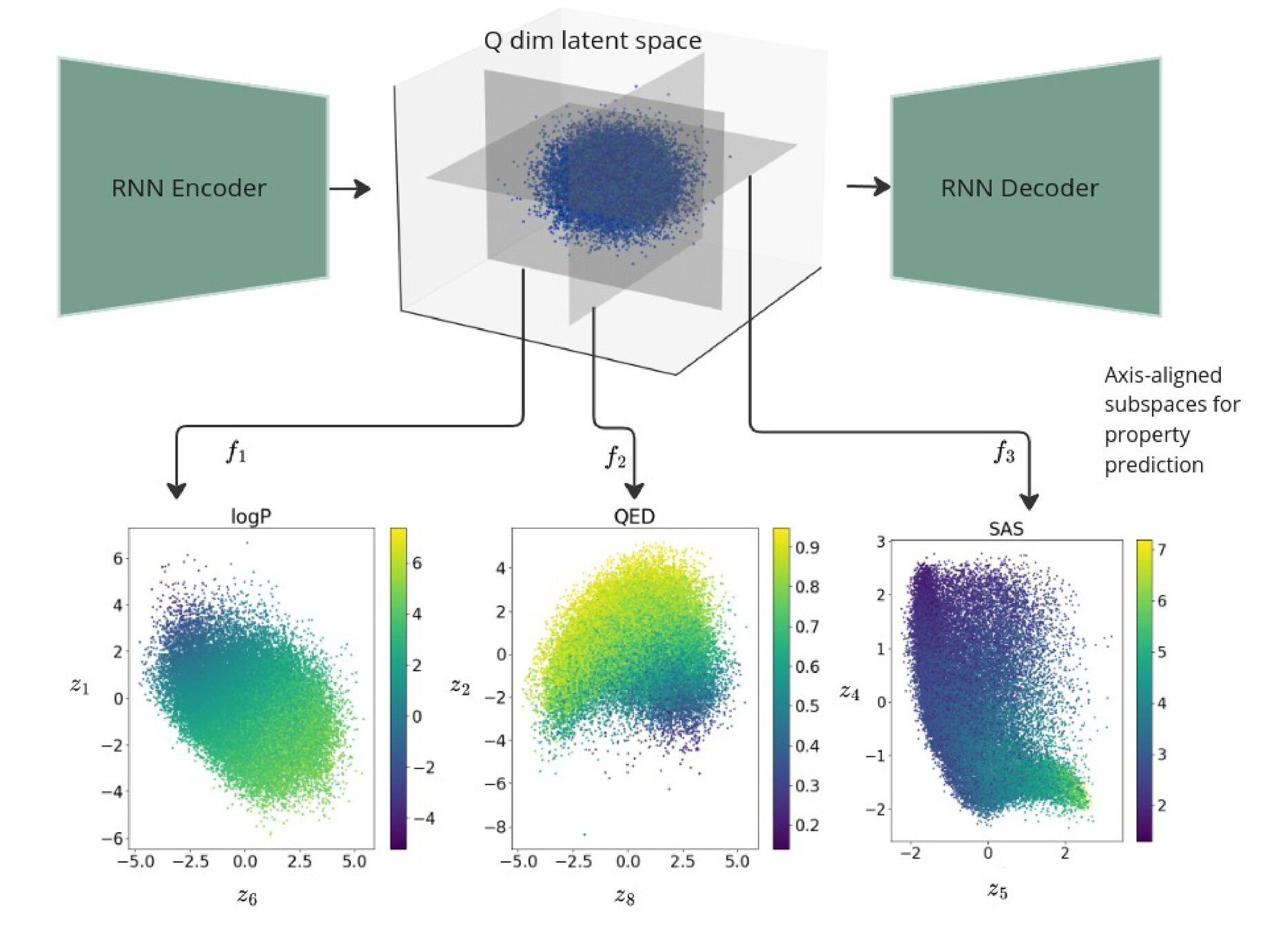
Gaussian process property decoders on the generative latent space
Recurrent VAE + Gaussian process decoders
Overall loss =
Q is the dimensionality of the latent space. The learnt lengthscales in each dimension indicate the influence of that dimension on the prediction.
Joint Model
Evolution of a 2d subspace of the latent space
Points shaded by actual QED (drug-likeness) scores
Can we do optimisations in a low dimensional subspace of the latent space and map back to the full latent space?
We really need extremely flexible inductive biases which adapt to the needs of the data - but you can just write down a new kernel function \(\longrightarrow\) much easier to explore non-stationary choices and parameterise them in interesting ways.
Hierarchical GPs also give rise to models with fat tailed predictive posteriors, this may be relevant in applications where we know our data to be heavy-tailed.
Hierarchical GPs are worth it only if you are in a weak data regime or in regimes with very high epistemic and aleatoric uncertainty. In these settings, a HGP will be much more robust to a canonical GP.
Summary, TLDR & Thanks
GPs can play the role of regularisers of the latent space in conditional generative models, the strength of the regularisation can be controlled by the choice of the kernel function.
email: vidrl@mit.edu / vr308@cam.ac.uk
twitter: @VRLalchand
Nested Sampling: The principle
Define a notion of prior volume, $$ X(\lambda) = \int_{\mathcal{L}(\theta) > \lambda} \pi(\theta)d\theta$$
The area/volume of parameter space "inside" a iso-likelihood contour
One can re-cast the multi-dimensional evidence integral as a 1d function of prior volume \( X\).
$$ \mathcal{Z} = \int \mathcal{L}(\theta)\pi(\theta)d\theta = \int_{0}^{1} \mathcal{L}(X)dX$$
The evidence can then just be estimated by 1d quadrature.
$$ \mathcal{Z} \approx \sum_{i=1}^{M}\mathcal{L_{i}}(X_{i} - X_{i+1})$$
Static Nested Sampling
Start with N "live" points \( \{\theta_{1}, \theta_{2}, \ldots, \theta_{N} \} \) sampled from the prior, \(\theta_{i} \sim p(\theta) \) , set \( \mathcal{Z} = 0\)
Skilling (2004)
for \( i = 1, \ldots, K\)
while stopping criterion is unmet do
Accumulate evidence, \( \mathcal{Z} = \mathcal{Z} + \mathcal{L}_{i}w_{i}\)
Evaluate stopping criterion, if triggered then break;
end
return set of saved points \(\{ \theta_{i}\}_{i=1}^{N + K} \), along with importance weights \( \{p_{i} \}_{i=1}^{N + K}\), and evidence \( \mathcal{Z} \)
Add final N live points to the "saved" list with:
# final slab of enclosed prior mass
\( \rightarrow \) hard problem
# why?
Prior Mass Estimation
Why is \( X_{i} \) set to \( e^{-i/N}\) where \(i\) is the iteration number and \(N\) is the number of live points.
(images from An Intro to dynamic nested sampling. Speagle (2017) )
Sampling from the constrained prior
Dynamic Nested Sampling. Speagle (2019)
At every step we need a sample \( \theta^{\prime}\) such that \( \mathcal{L_{\theta^{\prime}}} > \mathcal{L}_{i}\)
We could keep sampling uniformly from the prior and keep rejecting until we find one that meets the likelihood condition, but this takes too long when the likelihood threshold is high and there is a better way.
What if we could sample directly from the constrained prior?
New Directions
Neural encoder (parameteric)
Gaussian process (non-parameteric)
GPLVM: Generative Model with Sparse Gaussian processes
where,
Prior over latents:
Prior over inducing variables:
Conditional prior:
Data likelihood:
Stochastic Variational Evidence Lower bound
Stochastic variational inference for GP regression was introduced in Hensman et al (2013) (\( \mathcal{L}_{1}\) below). In this work we extend the SVI bound in two ways - we introduce the variational distribution over the unknown \(X\) and make \(Y\) multi-output.
ELBO:
Non-Gaussian likelihoods Flexible variational families Amortised Inference Missing data problems
Variational Formulation:
Vidhi Lalchand, Aditya Ravuri, Neil D. Lawrence. Generalised GPLVM with Stochastic Variational Inference. In International Conference on Artificial Intelligence and Statistics
(AISTATS), 2022
By Vidhi Lalchand


