


Vidhi Lalchand
Postdoctoral Fellow, Broad and MIT
Vidhi Lalchand
24-03-2025
Astro Data Science Reading Group at the Kavli Institute
stars
galaxies
|
Smith MJ, Geach JE. Astronomia ex machina: a history, primer and outlook on neural networks in astronomy. Royal Society Open Science. 2023 May 31;10(5):221454.
|
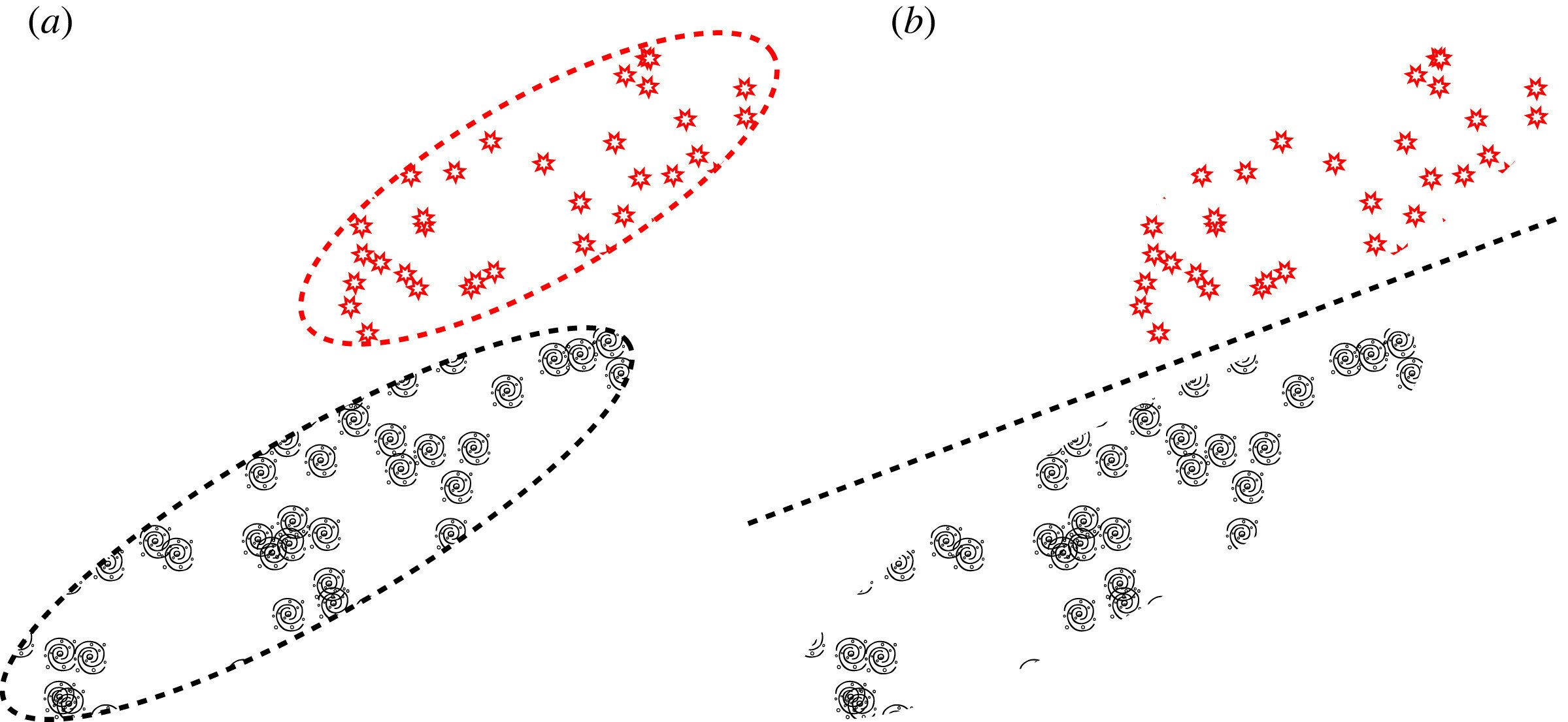
Generative models are powerful tools for embeddings discrete objects into a continuous space, thereby allowing one to simulate them.
Latent space
In (a), we see a generative model attempting to learn the probability distributions of the latent representation of a dataset that contains a set of galaxies and a set of stars. In (b), we see a discriminative model attempting to learn the boundary that separates the star and galaxy types.
|
Smith MJ, Geach JE. Astronomia ex machina: a history, primer and outlook on neural networks in astronomy. Royal Society Open Science. 2023 May 31;10(5):221454. |
Generative models are powerful tools for embeddings discrete objects into a continuous space, thereby allowing one to simulate them.
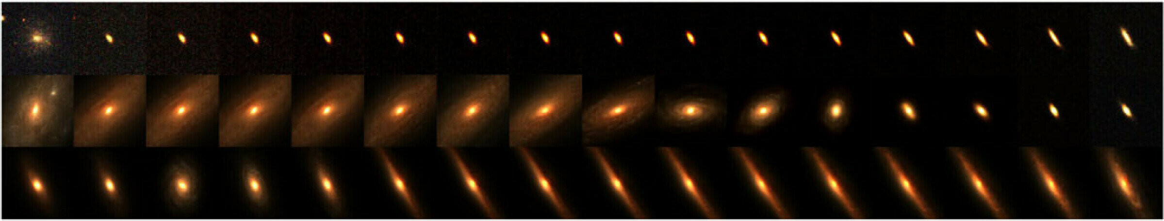
Latent space
Interpolating between the continuous representation of astronomical objects in latent space
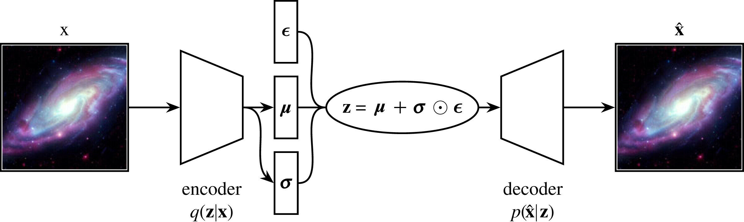
Typical autoencoder style architecture of generative models
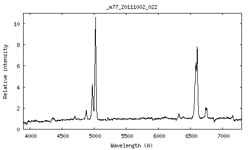
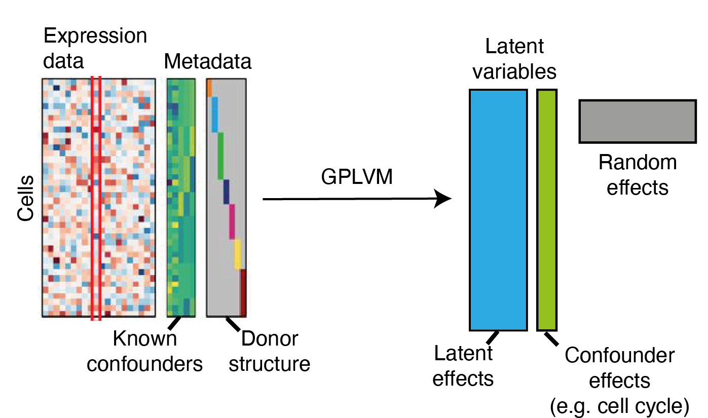
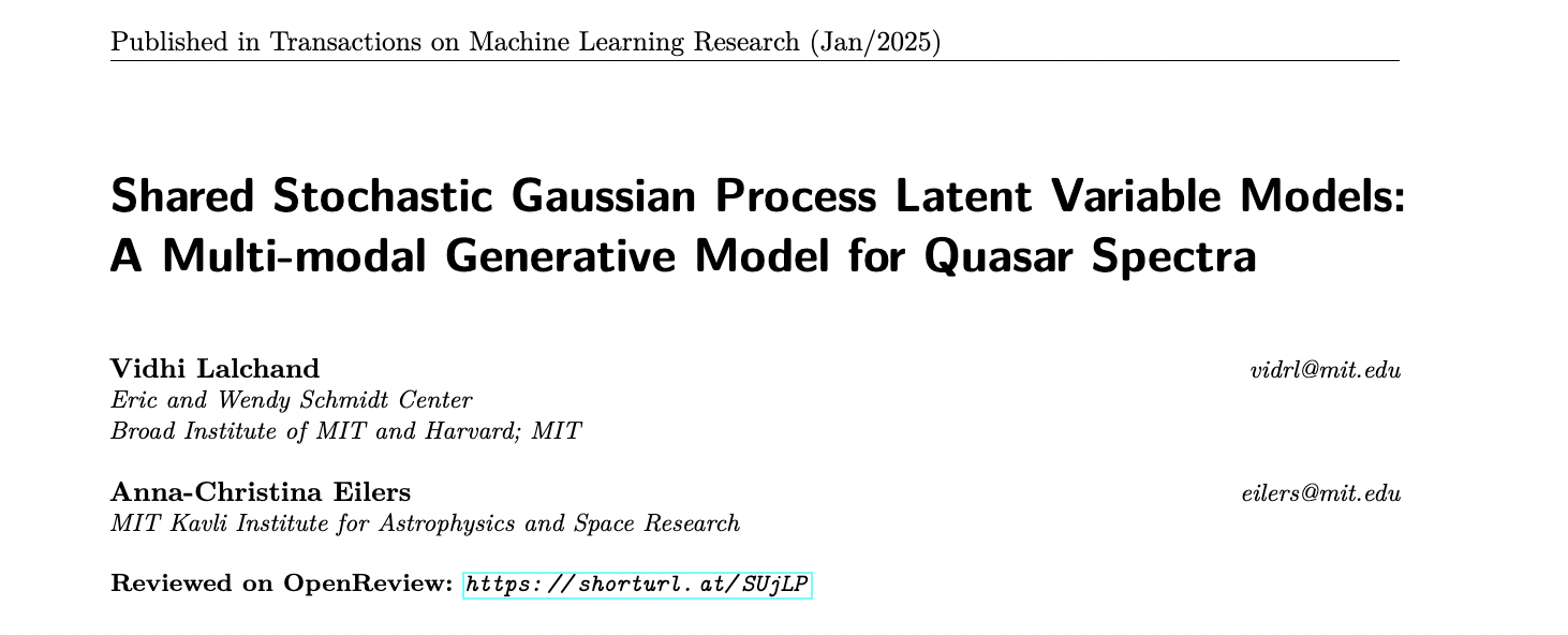
Aim: To build a joint generative model for quasar spectra and their black hole engines using a non-parametric modelling framework based on Gaussian processes.
[Lbol, Bhm, Eddington ratio, Redshift]
For each quasar we have,
Observation space 1 Observation space 2
\(N\) = ~23,000 quasars, \(D\) = 590 (spectral pixels), \(L\) = 4 (scientific labels)
Data:
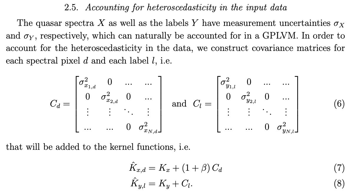
- Heteroscedasticity: The datasets have been constructed by combining measurements from different instruments / telescopes. Hence, due to the different redshift, the quasars cover slightly different rest-frame wavelengths.
- Missing spectral regions: The rectangular dataset is prepared by shifting the quasars into a restframe wavelength space and re-binning into a common wavelength grid with a fixed pixel scale. Any unobserved pixels are set to NaNs.
We need a probabilistic model which can handle these challenges in a principled and rigorous way.
Non-linear mapping / Decoder
X
Y
Z
Hidden / Latent variables per data point
Observed spectra & Labels
\( N \times D N \times L\)
\( N \times Q \)
Gaussian processes are a powerful non-parametric paradigm for performing probabilistic regression.
We need to understand the notion of distribution over functions.
What is a GP?
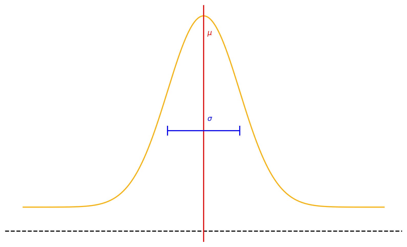
A sample from a \(k\)-dimensional Gaussian \( \mathbf{x} \sim \mathcal{N}(\mu, \Sigma) \) is a vector of size \(k\).
$$ \mathbf{x} = [x_{1}, \ldots, x_{k}] $$
The mathematical crux of a GP is that \( [f(x_{1}), f(x_{2}), f(x_{3}),....., f(x_{n})]\) is just a N-dimensional multivariate Gaussian \( \mathcal{N}(\mu, K) \).
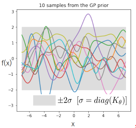
A GP is an infinite dimensional analogue of a Gaussian distribution \( \rightarrow \) a sample from it is a vector of infinite length?
But at any given point, we only need to represent our function \( f(x) \) at a finite index set \( \mathcal{X} = [x_{1},\ldots, x_{500}]\). So we are interested in our long function vector \( [f(x_{1}), f(x_{2}), f(x_{3}),....., f(x_{500})]\).
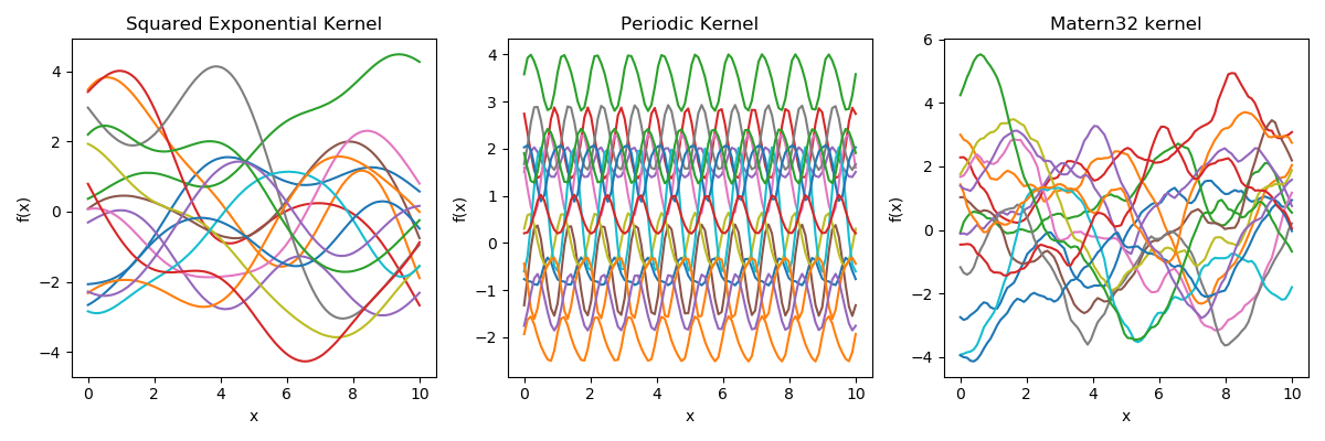
The kernel function \( k(x,x')\) is the heart of a GP, it controls all of the inductive biases in our function space like shape, periodicity, smoothness.
prior over functions \( \rightarrow \)
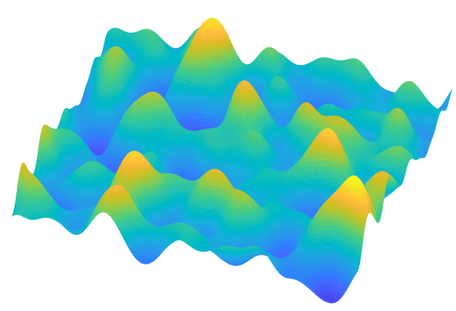
Sample draws from a zero mean GP prior under different kernel functions.
In reality, they are just draws from a multivariate Gaussian \( \mathcal{N}(0, K)\) where the covariance matrix has been evaluated by applying the kernel function to all pairs of data points.
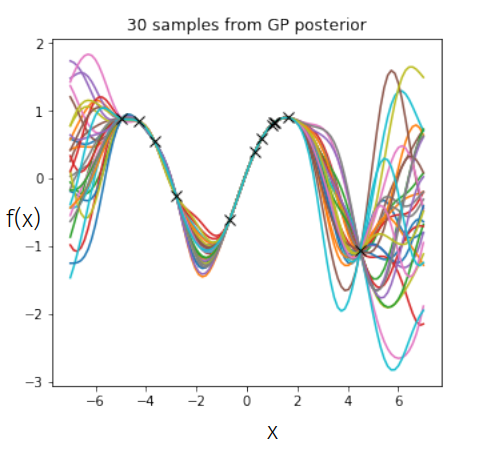
1. Given some noisy data \( \bm{y} = \lbrace{y_{i}}\rbrace_{i=1}^{N} \) at \( X = \{ x_{i}\}_{i=1}^N\) input locations.
2. You model your data as coming from a hidden function \( f\) corrupted by Gaussian noise.
$$ \bm{y} = f(X) + \epsilon, \hspace{10pt} \epsilon \sim \mathcal{N}(0, \sigma^{2})$$
Data Likelihood: \( \hspace{10pt} y|f \sim \mathcal{N}(f(x), \sigma^{2}) \)
Prior over functions: \( f|\theta \sim \mathcal{GP}(0, k_{\theta}) \)
(The choice of kernel function \( k_{\theta}\) controls how your functions space looks.)
Learning Step in Regression:
Learning in Gaussian process models occurs through the maximisation of the marginal likelihood w.r.t the kernel hyperparameters.
Data likelihood
Prior
Learning Step (when X is hidden/ latent):
Extending GPs to the latent variable set-up introduces two fundamental changes:
1. We need to account for the multi-output space, the targets are not scalars but have \(D\) dimensions.
2. The inputs (assumed to be fixed in regression) are hidden and need to be learnt.
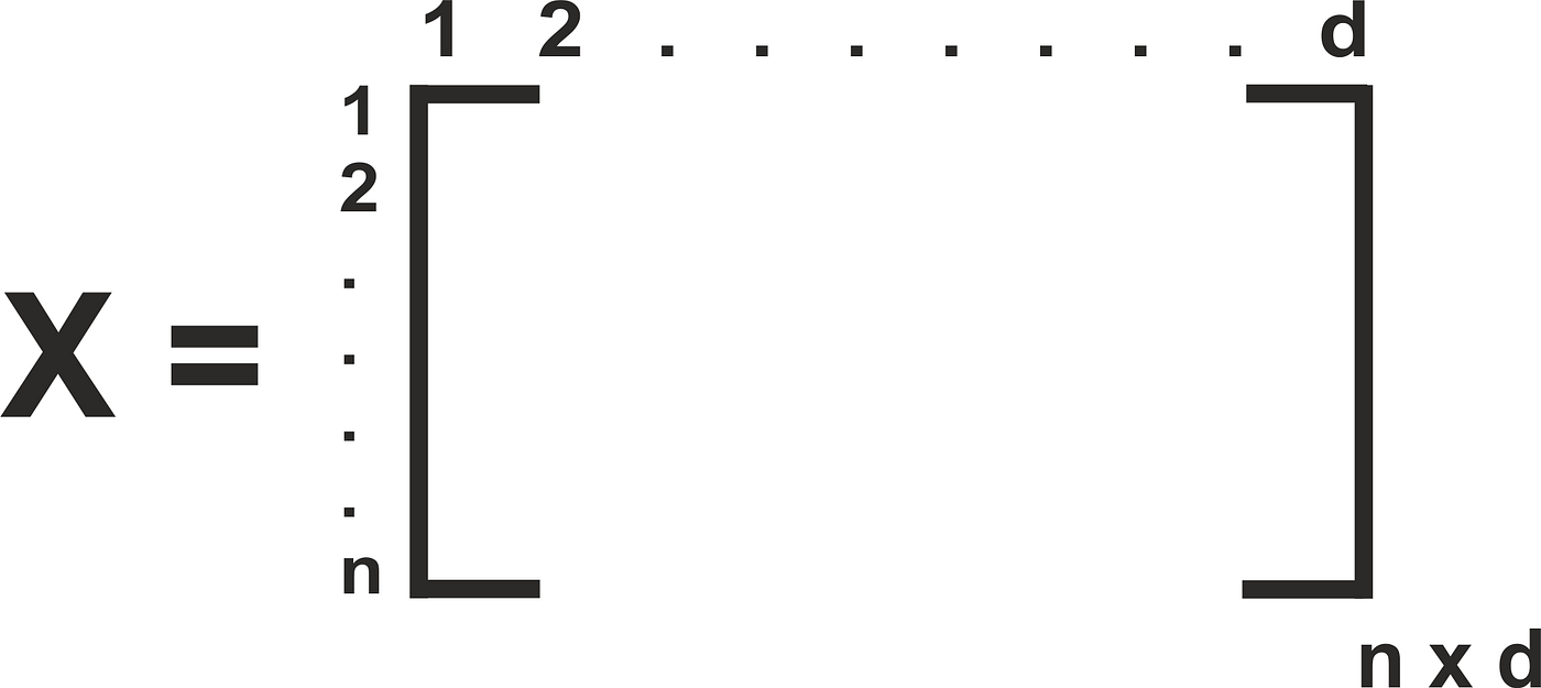
Gaussian processes can also be used in contexts where the observations are a gigantic data matrix \( Y \equiv \{ y_{n}\}_{n=1}^{N}, y_{n} \in \mathbb{R}^{D}\). \(D\) can be pretty big \(\approx 1000s\).
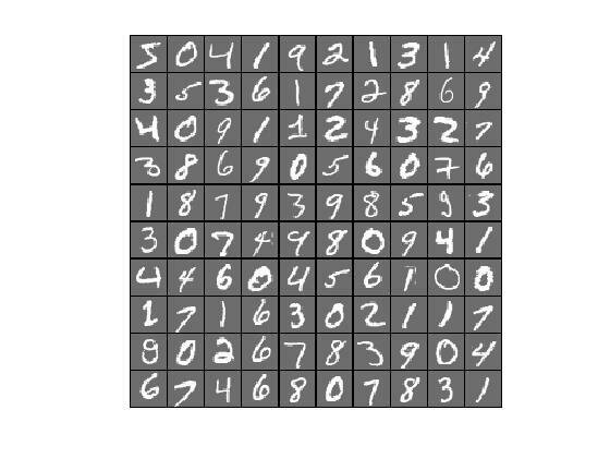
Imagine a stack of images, where each image has been flattened into a vector of pixels and stacked together rowise in a matrix.
28
28
n = number of images
d = 784
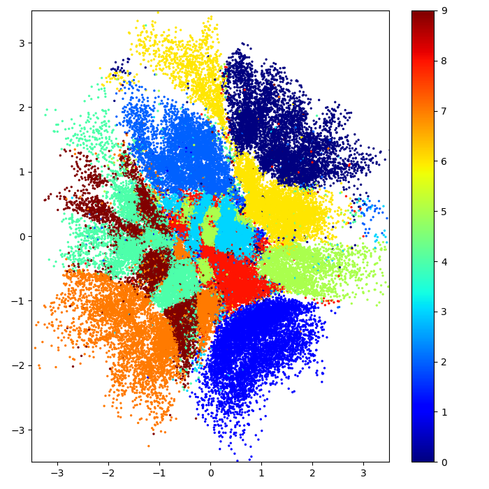
Given: High dimensional training data \( Y \equiv \{\bm{y}_{n}\}_{n=1}^{N}, Y \in \mathbb{R}^{N \times D}\)
Learn: Low dimensional latent space \( X \equiv \{\bm{x}_{n}\}_{n=1}^{N}, X \in \mathbb{R}^{N \times Q}\)
\( Q << D\)
Given: High dimensional training data \( Y \equiv \{\bm{y}_{n}\}_{n=1}^{N}, Y \in \mathbb{R}^{N \times D}\)
Learn: Low dimensional latent space \( X \equiv \{\bm{x}_{n}\}_{n=1}^{N}, X \in \mathbb{R}^{N \times Q}\)
GP prior over mappings
(per dimension, \(d\))
Choice of \( \mathbf{K}\) induces non-linearity
GP marginal likelihood
Optimisation problem:
The Gaussian process decoder
2d latent space
High-dimensional data space
. . .
. . .
N
D
\( X \in \mathbb{R}^{N \times Q}\)
\( F \in \mathbb{R}^{N \times D}\)
\( Y \in \mathbb{R}^{N \times D}\)
Data Likelihood:
Prior structure:
The data are stacked row-wise but modelled column-wise, each column with a GP.
\(X\)
\(x_{n}\)
Given: High dimensional training data \( Y \equiv \{\bm{y}_{n}\}_{n=1}^{N}, Y \in \mathbb{R}^{N \times D}\)
Learn: Low dimensional latent space \( X \equiv \{\bm{x}_{n}\}_{n=1}^{N}, X \in \mathbb{R}^{N \times Q}\)
Observed space
Gaussian Process Mapping
Model:
The Gaussian process mapping
2d latent space
High-dimensional data space
. . .
. . .
N
D
\( X\in \mathbb{R}^{N \times Q}\)
\( f_{d} \sim \mathcal{GP}(0,k_{\theta})\)
\( Y \in \mathbb{R}^{N \times D} (= F + noise)\)
The latents are continuous values, hence, the most popular choice of kernel function is the RBF kernel with lengthscale per dimension.
The behaviour of the lengthscales during training achieves sparsity - it prunes away redundant dimensions in the latent space.
Parameteric VAEs
Auto-encoded GPLVM
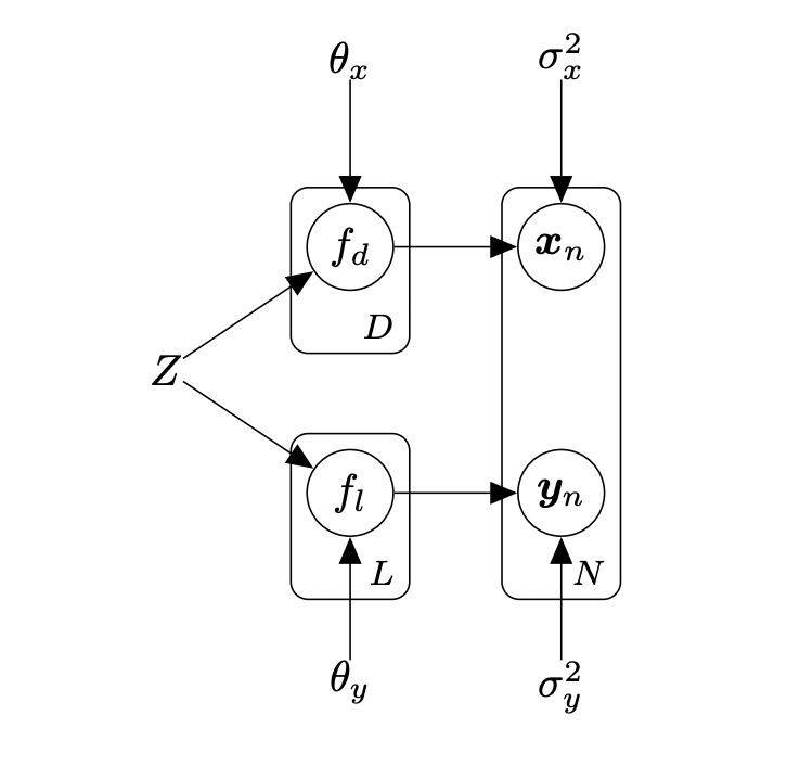
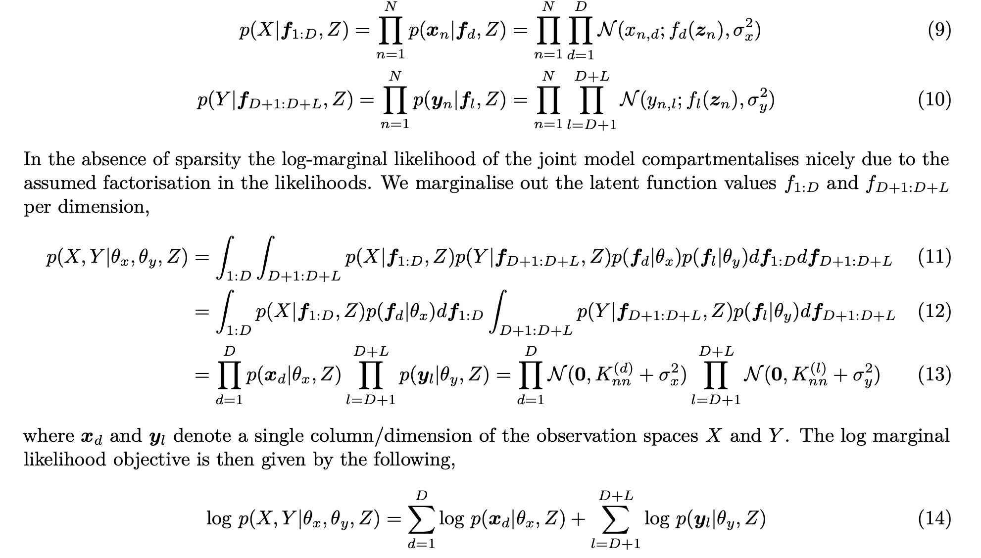
Crux: We use two groups of GPs to model the spectra and the labels, however, they share the same latent space.
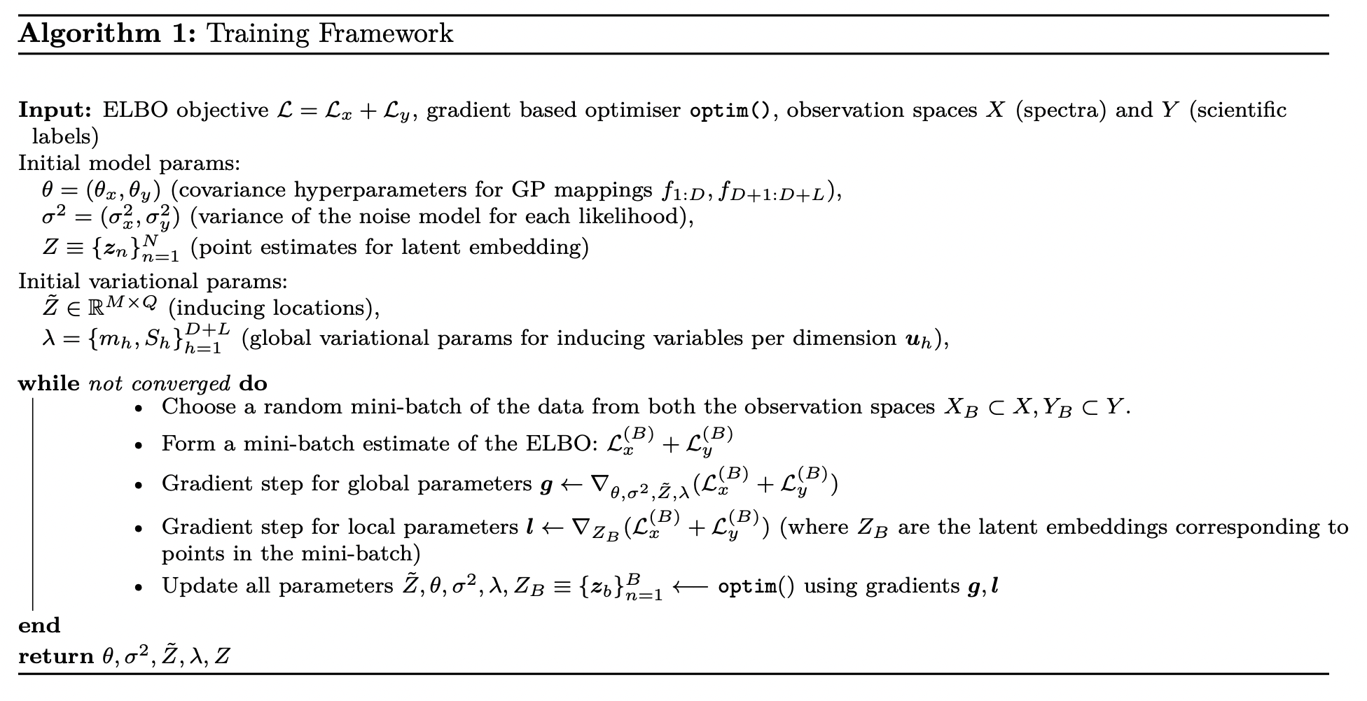
Optimisation objective:
Crux: We use two groups of GPs to model the spectra and the labels, however, they share the same latent space.
Optimisation objective:
Nice compartmentalisation of the GP marginal likelihood
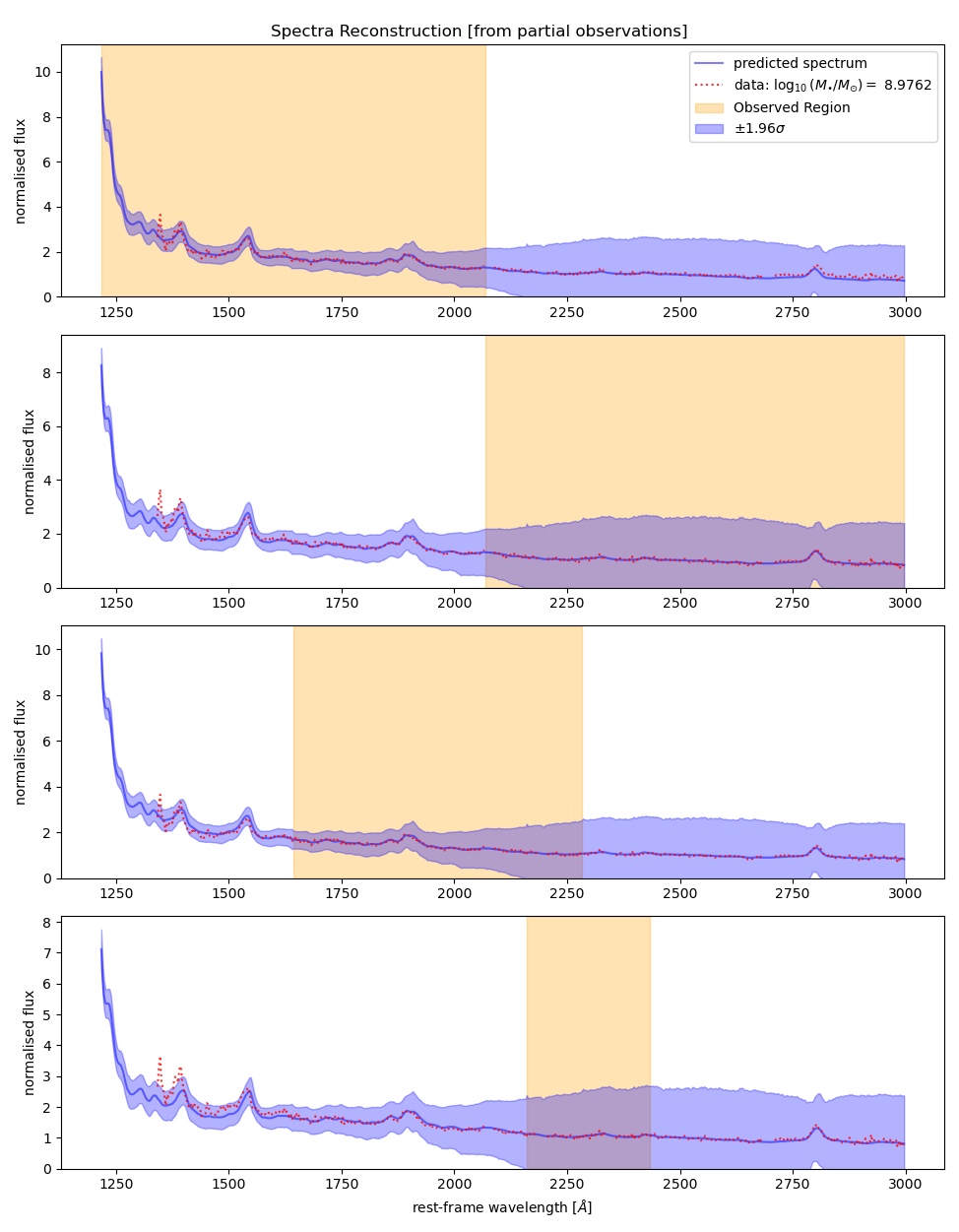
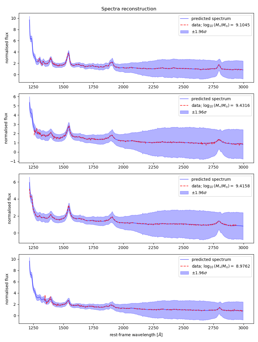
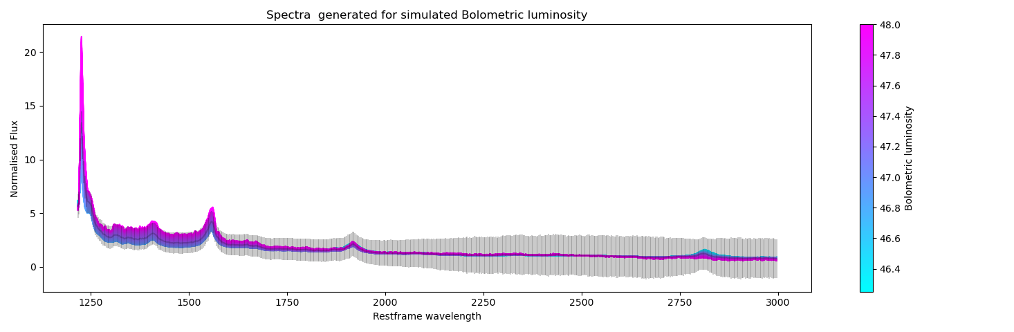
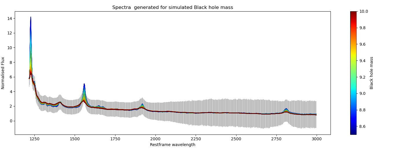
higher uncertainty bands at higher wavelengths (epistemic uncertainty)
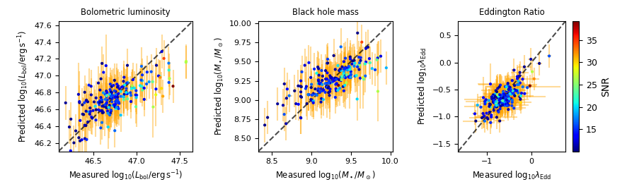
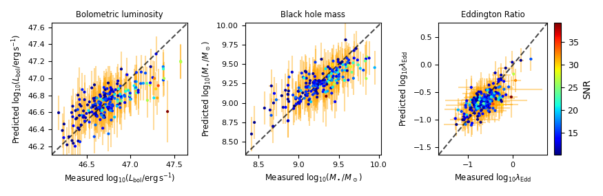
Quantitatively we measure the reconstruction accuracy using error - deviation of the red line from the blue.
The log predictive density captures how well the ground truth is contained within the uncertainty bounds.
\([f_{1}(z_{i}), f_{2}(z_{1}), f_{3}(z_{i}), \ldots f_{D}(z_{i})]\)
Prediction for object \(i\)
Evaluation of \(D\) GPs at the latent vector \( \color{blue}z_{i}\)
gt: ground truth
est: estimated
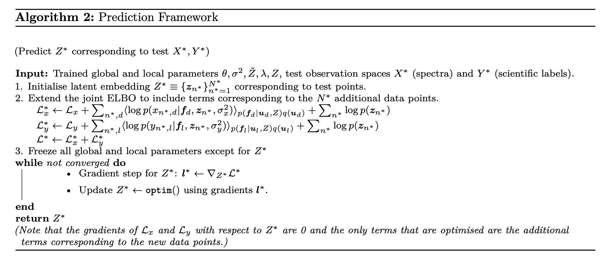
\(X^{*}\)
\(Z^{*}\)
\(Y^{*}\)
spectra
scientific labels
latents
Step 1: Learn latent \(Z^{*}\) from ground truth spectra or both spectra and labels. (Inference step)
Step 2: Decode \(Z^{*}\) using the GPs \(f_{l}\) to predict the labels.
(Cross-modal prediction)
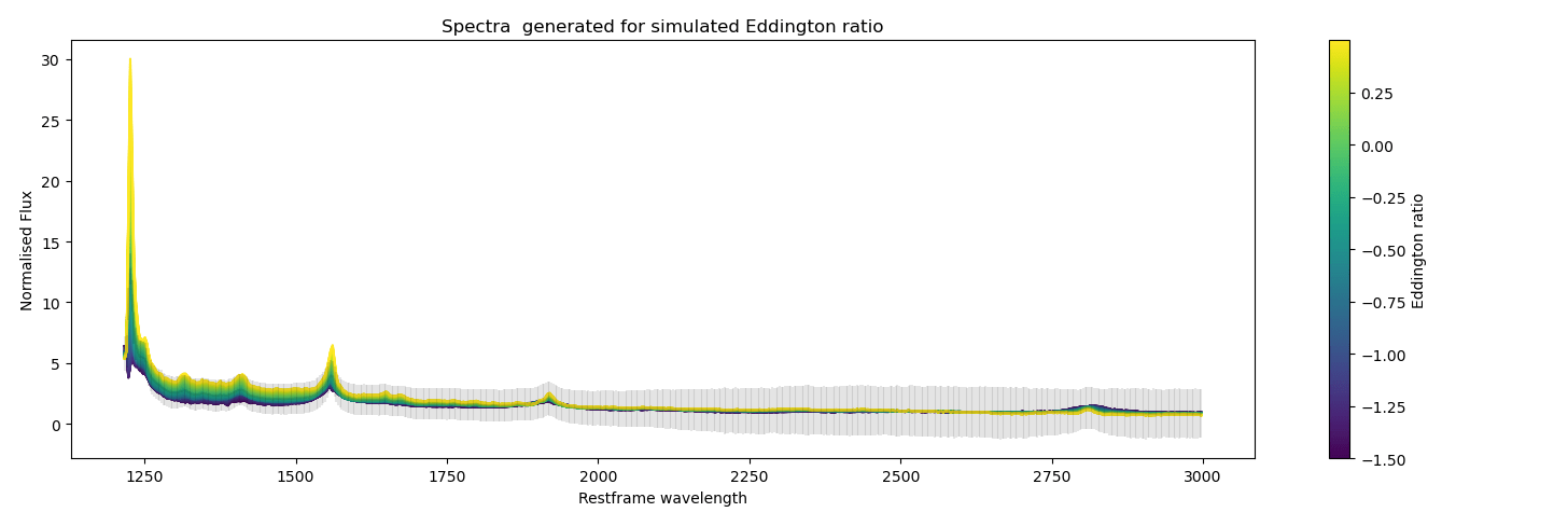
An experiment demonstrating cross-modal prediction \(Y^{*} \longrightarrow Z^{*} \longrightarrow X^{*}\) . In the plots we show generated quasar spectra for simulated labels for black hole mass, bolometric luminosity and Eddington ratio. In each plot we vary the respective scientific label in a reasonable range (shown by the range on the colorbar) while keeping the other labels to fixed values.
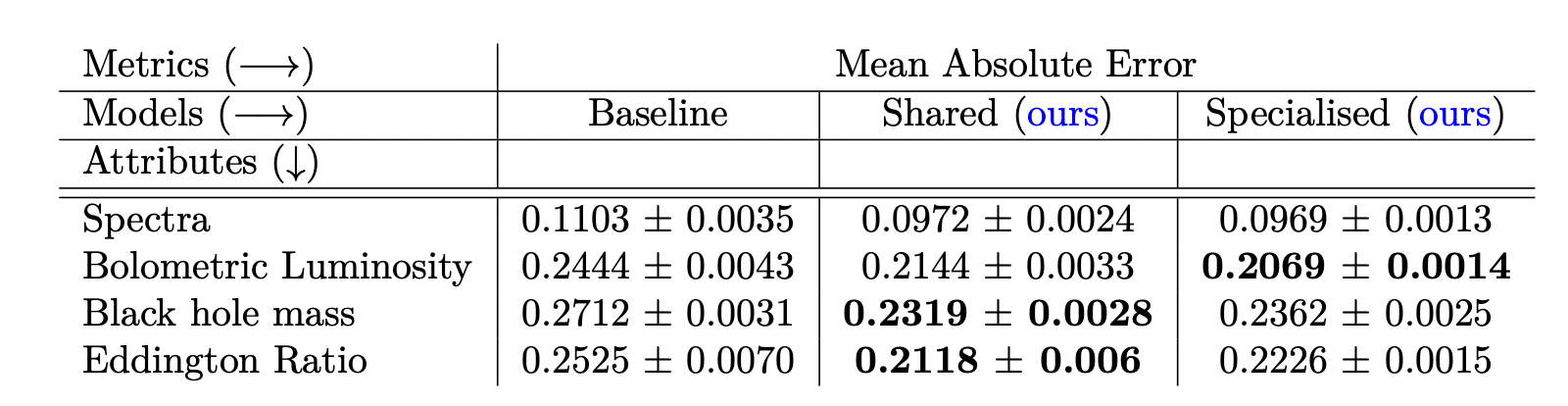
Reconstruction error on unseen objects across all modalities (lower is better).
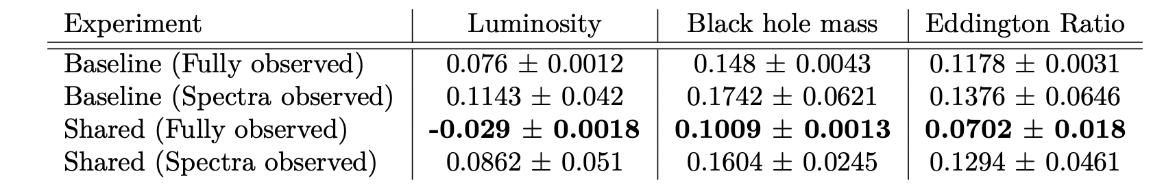
Uncertainty quantification measured through negative log predictive density on unseen objects (lower is better).
cross-modal
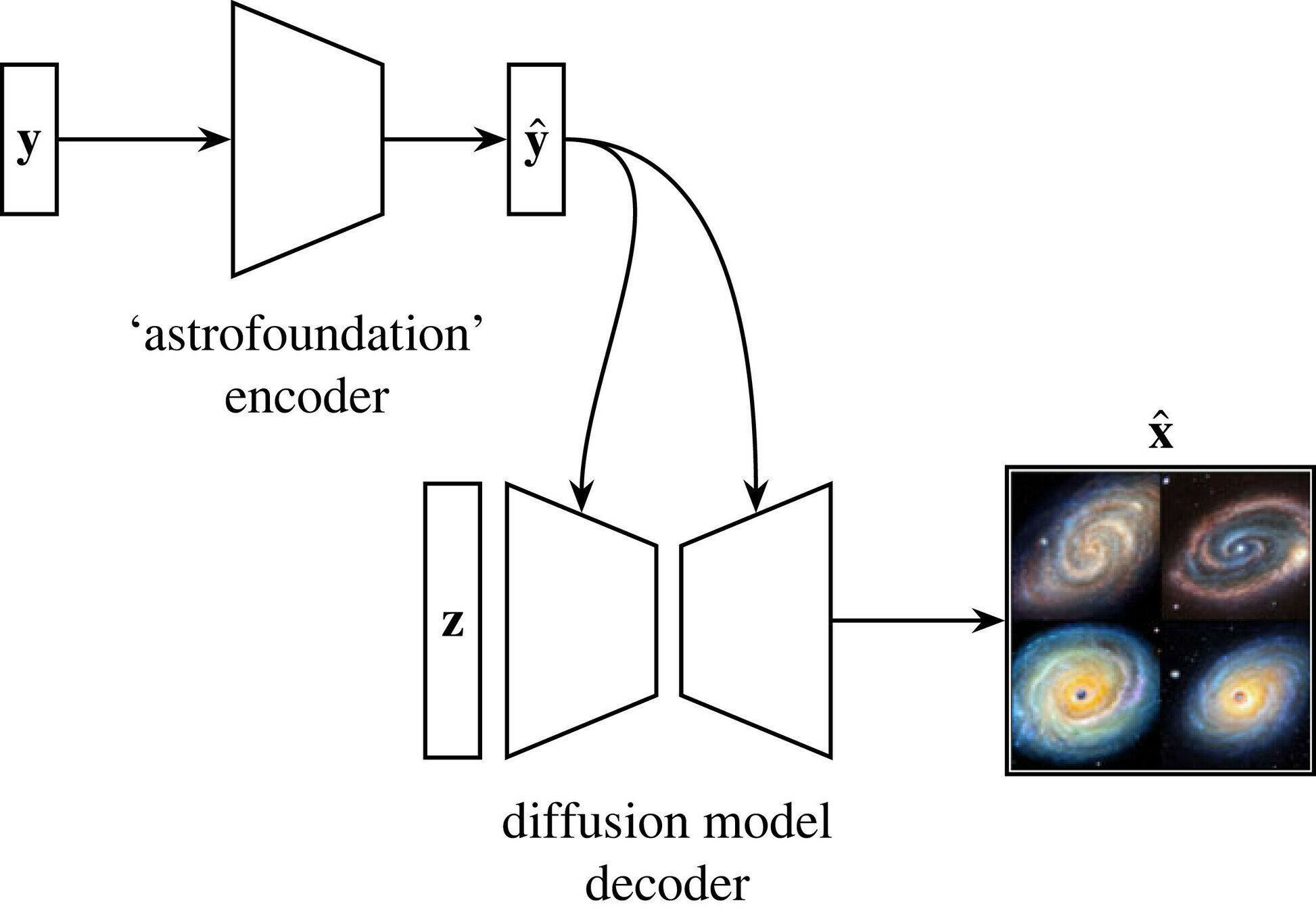
Can we learn universal task-agnostic latent vectors in a self-supervised way; these latents can be used down-stream in smaller, custom models for downstream research.
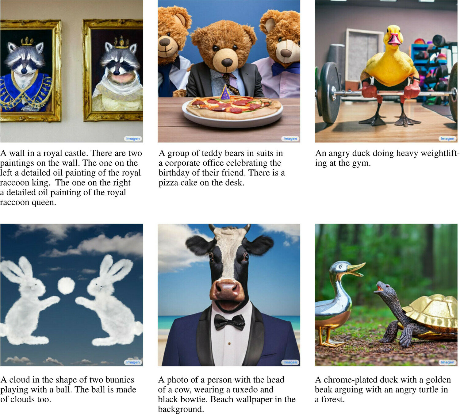
IMAGEN: Text-to-image foundation model
Conditional Generation using a frozen pre-trained foundation model
frozen weights
Thank you!
Prof. Anna-Christina Eilers
eilers@mit.edu
My contact:
vidrl@mit.edu
vr308@cam.ac.uk
@VRLalchand
Summary
By Vidhi Lalchand


