


Vidhi Lalchand
Postdoctoral Fellow, Broad and MIT
Jan-Feb 2021
Fergus Simpson, Vidhi Lalchand, Carl E. Rasmussen
Background: Gaussian Processes
Gaussian Processes offer a powerful, Bayesian, non-parametric paradigm for learning functions.
Background: Gaussian Processes
Gaussian Processes offer a powerful, Bayesian, non-parametric paradigm for learning functions.
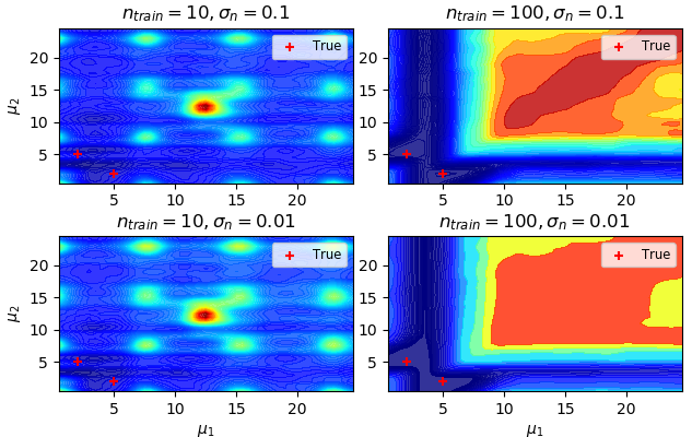
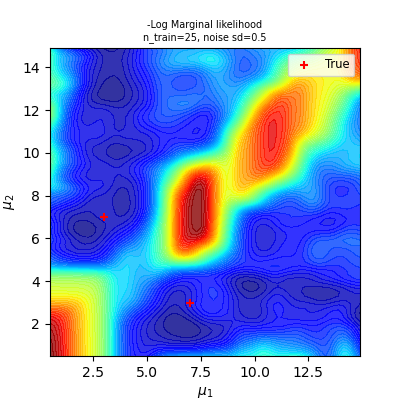
Conventionally, learning occurs via maximisation of the marginal likelihood
Objectives
Objectives
Learning with Spectral Mixture Kernels
Learning with Spectral Mixture Kernels
Marginalised Gaussian Processes
Generative Model
Marginalised Gaussian Processes
Generative Model
Predictions
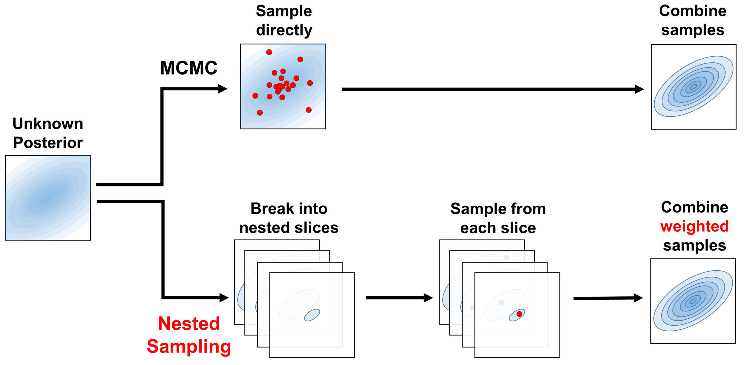
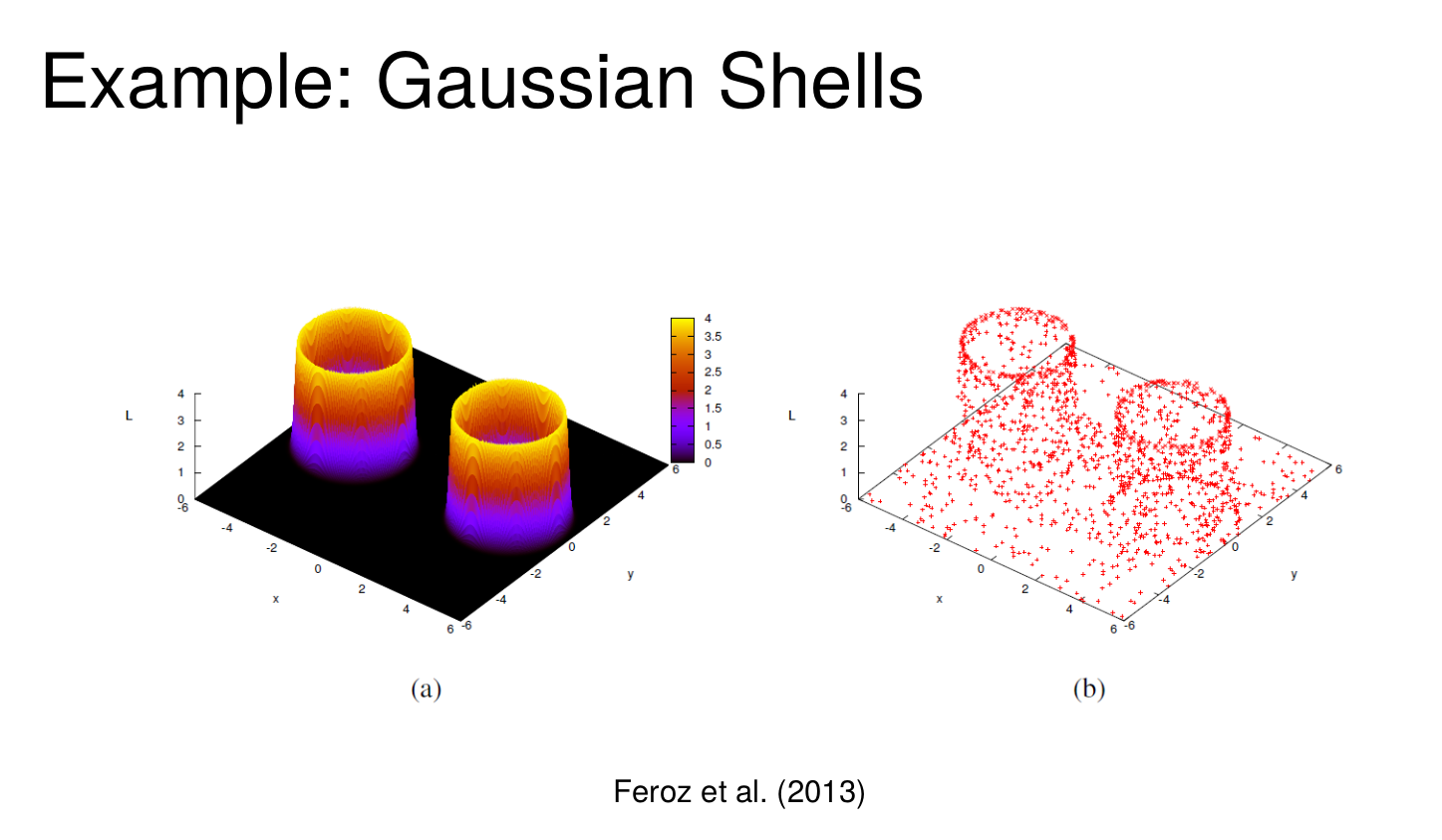
Overview: Nested Sampling
Speagle JS. dynesty: a dynamic nested sampling package for estimating Bayesian posteriors and evidences. Monthly Notices of the Royal Astronomical Society. 2020 Apr;493(3):3132-58.
Overview: Nested Sampling
Speagle JS. dynesty: a dynamic nested sampling package for estimating Bayesian posteriors and evidences. Monthly Notices of the Royal Astronomical Society. 2020 Apr;493(3):3132-58.
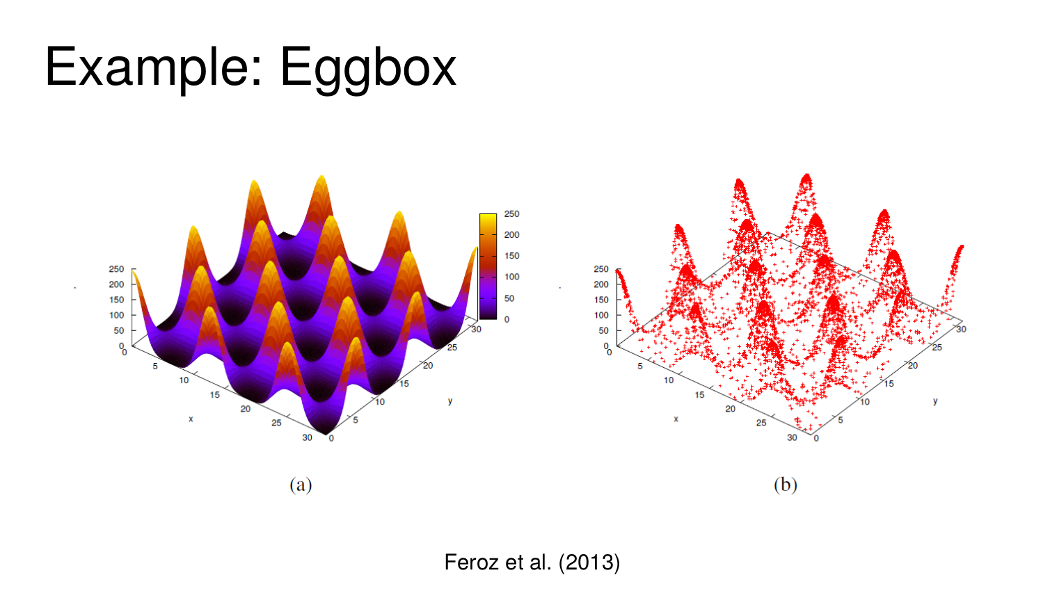
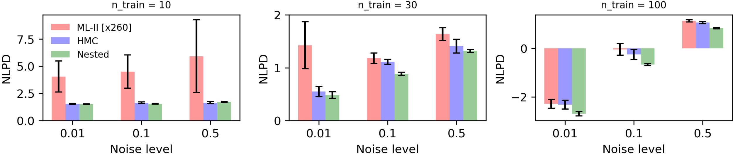
Synthetic Experiments
Synthetic Experiments
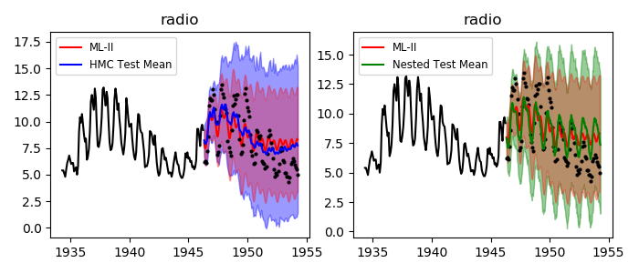
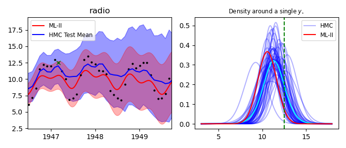
Time-series prediction (1d)
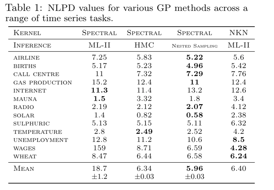
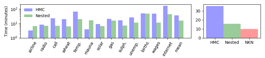
Time series benchmarks
Time series benchmarks
Time-series prediction (1d)
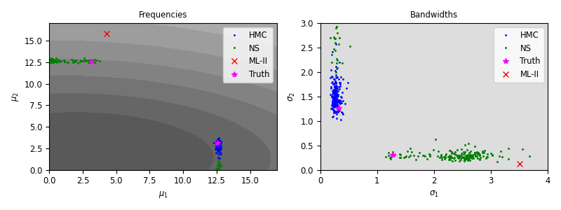
Why is it better?
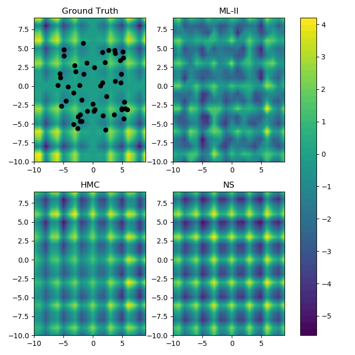
Pattern Prediction (2d)
Train: 50 points chosen randomly and uniformly between [-6 x 6] grid.
Test: [-10 x 10] grid of 400 points.
NLPD
ML-II: 216
Hamiltonian Monte Carlo: 2.56
Nested Sampling : 2.62
Summary
Summary
Marginalised GPs give robust prediction intervals by accounting for hyperparameter uncertainty. Their advantage over ML-II become particularly pronounced when expressive kernels with several hyperparameters are used or where the training data is either sparse or noisy.
Thank you!
By Vidhi Lalchand


