

Vidhi Lalchand
Postdoctoral Fellow, Broad and MIT
Gaussian Process Parameterised Covariance Kernels for Non-stationary Regression
Vidhi Lalchand\(^{1}\), Talay Cheema\(^{1}\), Laurence Aitchison\(^{2}\), Carl E. Rasmussen\(^{1}\)
Motivation: Non-Stationary Kernels
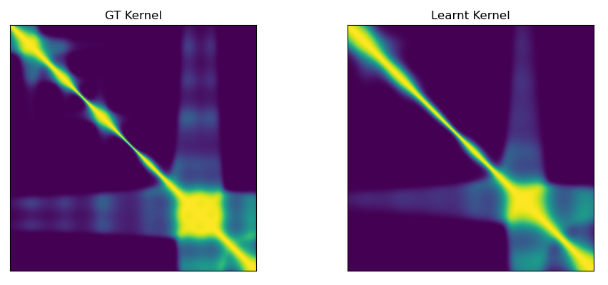
Learning a non-stationary kernel (1d)
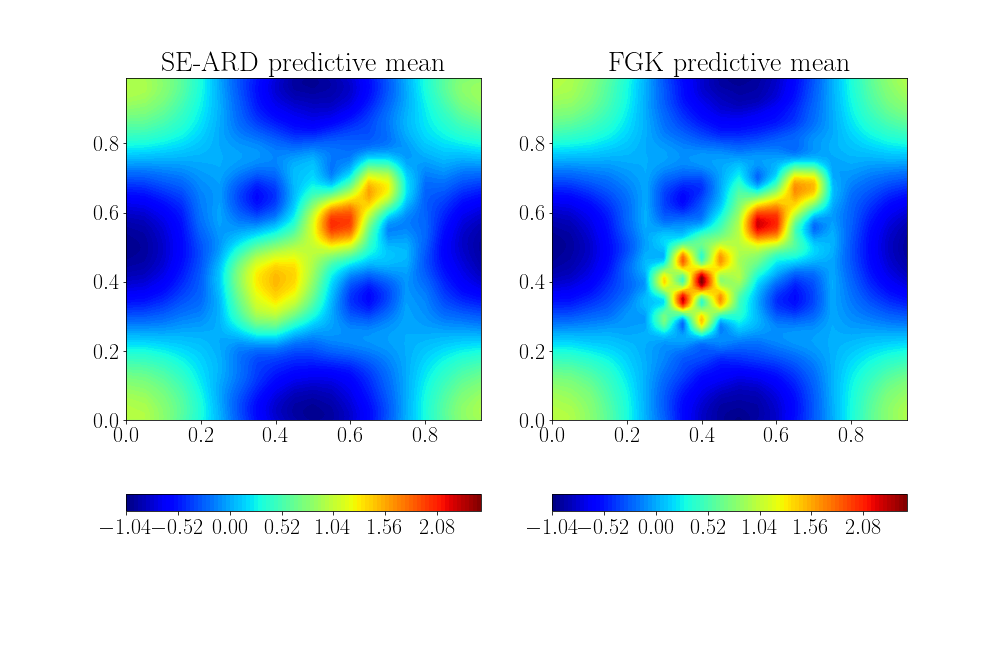
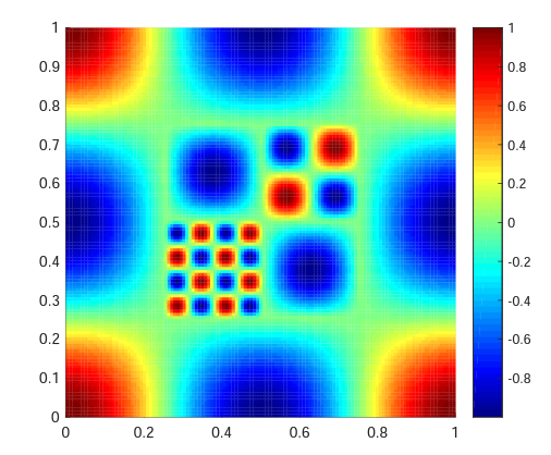
Reconstructing a 2d non-stationary surface
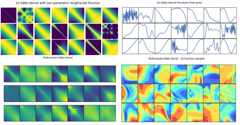
A large cross-section of Gaussian process literature uses universal kernels like the squared exponential (SE) kernel along with automatic revelance determination (ARD) in high-dimensions. The ARD framework in covariance kernels operates by pruning away extraneous dimensions through contracting their inverse-lengthscales. This works considers probabilistic inference in the factorised Gibbs kernel and the multivariate Gibbs kernel with input-dependent lengthscales. These kernels allow for non-stationary modelling where samples from the posterior function space ``adapt" to the varying smoothness structure inherent in the ground truth. We propose parameterizing the lengthscale function of the factorised and multivariate Gibbs covariance function with a latent Gaussian process defined on the same inputs.
We use MAP inference with a GP prior over the lengthscale process to recover the ground truth kernel (left) with radomly distributed training data points.
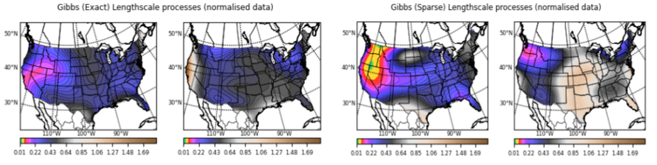
Modelling Precipitation Across Continental United States
Approximate posterior predictive means for the 2d surface using 250 inducing points. The factorised Gibbs kernel (FGK) adapts to the lower length-scale behaviour in the central areas while the standard SE-ARD kernel is forced to subscribe to a single lengthscale.
University of Cambridge\(^{1}\), University of Bristol\(^{2}\)
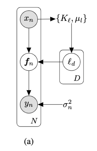
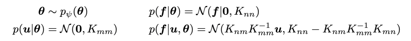
The hierarchical GP framework is given by,
where \(K_{mm}\) denotes the covariance matrix computed using the same kernel function \(k_{\theta}\) on inducing locations \(Z\) as inputs; the likelihood factorises across data points, \(p(\bm{y}|\bm{f}) = \prod_{i=1}^{N}p(y_{i}|f_{i}) = \mathcal{N}(\bm{y}|\bm{f}, \sigma_{n}^{2}\mathbb{I})\) and \(\psi\) denote parameters of the hyperprior. The joint model is given by, \(p(\bm{y},\bm{f},\bm{u},\bm{\theta}) = p(\bm{y}|\bm{f})p(\bm{f}|\bm{u},\bm{\theta})p(\bm{u}|\bm{\theta})p(\bm{\theta}) \).
The standard marginal likelihood \(p(\bm{y}) = \int p(\bm{y}|\bm{\theta})p(\bm{\theta})d\bm{\theta}\) is intractable. The inner term \(p(\bm{y}|\bm{\theta})\) is the canonical marginal likelihood \(\mathcal{N}(\bm{y}|\bm{0}, K + \sigma^{2}_{n}\mathbb{I})\) in the exact GP case and is approximated by a closed-form evidence lower bound (ELBO) in the sparse GP case for a Gaussian likelihood. The sparse variational objective in the extended model augments the ELBO with an additional term to account for the prior over hyperparameters, \(\log p(\bm{y}, \bm{\theta}) \geq \mathcal{L}_{sgp} + \log p_{\psi}(\bm{\theta})\).
By Vidhi Lalchand


