
Ishanu Chattopadhyay PRO
ML | Data Science Biomedical Informatics | Social Science | Assistant Professor
Ishanu Chattopadhyay, PhD
Assistant Professor of Biomedical Informatics & Computer Science
University of Kentucky
| reliten | gunlaw | abany | --- | grass | |
|---|---|---|---|---|---|
| Person 1 | |||||
| Person 2 | |||||
| --- | |||||
| Person m |
observables
samples
Distributions over alphabet \(\Sigma^i\)
Individual Predictor (CIT)
cross-talk
Tension between predicted and observed distribution drives change
Example
GSS topic: There should be more gun-control
\(\psi^i\)
| strongly agree | agree | neutral | disagree | strongly disagree |
\(\phi\) estimates \(\psi\)
Examples: GSS, ANES, WVS, ESS, Eurobarometer, Afrobarometer, Asian Barometer etc
group
individual
estimate is always a non-empty non-degenerate distribution
missing observation
*Hothorn, Torsten, Kurt Hornik, and Achim Zeileis. "Unbiased recursive partitioning: A conditional inference framework." Journal of Computational and Graphical statistics 15, no. 3 (2006): 651-674.
emergent macro-structure
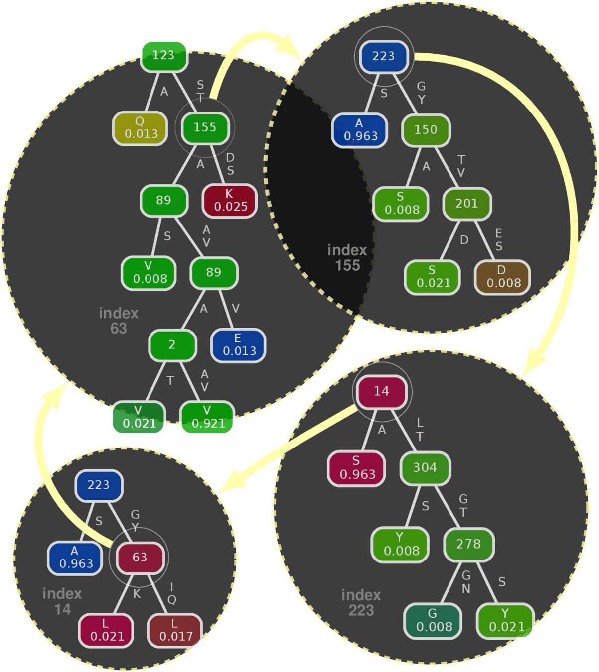
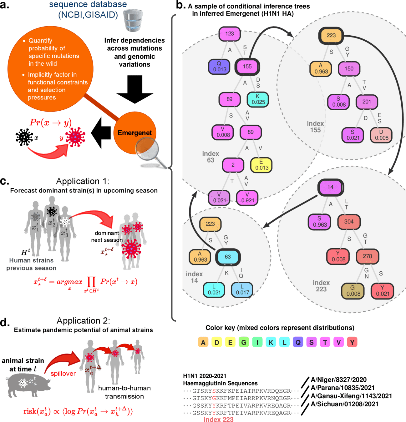
Component predictor (Conditional Inference Tree*)
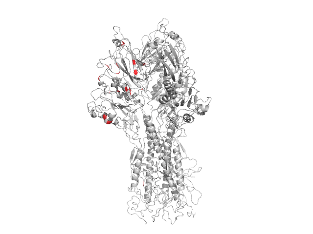
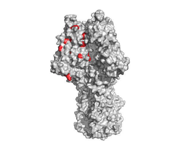
Example: Influenza A HA protein
Recursive
LSM
forest
Revealing Emergent Cross-talk
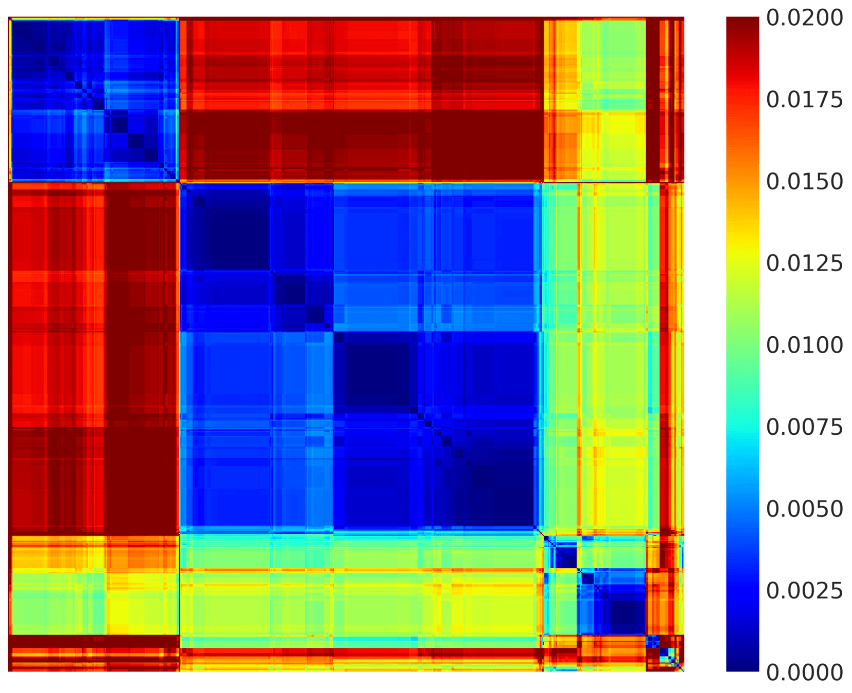
where \(D_{JS}(P\vert \vert Q)\) is the Jensen-Shannon divergence.
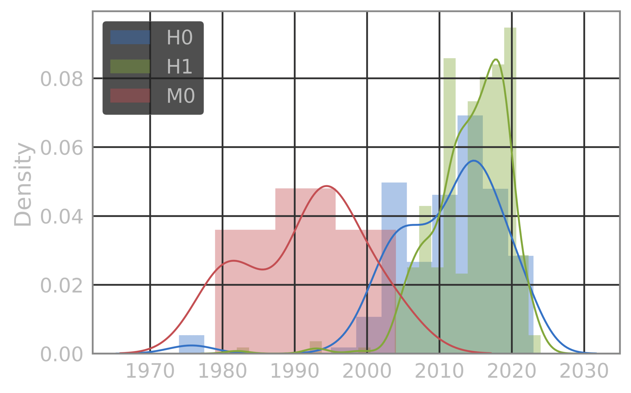
H0
H1
M0
The three bovine sequences are not part of these clusters (these are all human ICV HE), but we can still compute the distance of the individual human sequences to each of the three bovine strains. And the cluster they come closest to.. Pretty clearly is the one labelled as M0. The other clusters are labeled H0 and H1.
Distance of bovine sequences to M0 cluster
'C/Miyagi/2/94', 'C/Saitama/2/2000', 'C/Yamagata/3/2000', 'C/Miyagi/7/93', 'C/Miyagi/4/96', 'C/Saitama/1/2004', 'C/Miyagi/7/96', 'C/Greece/1/79', 'C/Yamagata/5/92', 'C/Miyagi/3/93', 'C/Miyagi/4/93', 'C/Kyoto/41/82', 'C/Nara/82', 'C/Hyogo/1/83', 'C/Miyagi/1/94', 'C/Miyagi/6/93', 'C/Miyagi/3/94', 'C/Mississippi/80', 'C/Yamagata/26/2004', 'C/Mississippi/80'
Suggests movement from M0 to H0 to H1
| M0 | -64.251 |
|---|---|
| H0 | -32.586 |
| H1 | -15.964 |
Fitness calculations are based on the Emergenet model, and correspond to the estimate loglikelihood of a strain NOT PERTURBING out of the cluster. Thus the H1 cluster is the most "fit", where the strains have moved over time, and is also the largest in the data. Overlap on the collection times between H0 and H1 implies this is not simply a collection bias effect (the sizes of the clusters). This has resulted in the strain disappearing from humans, as the virus found a more fit niche on the landscape.
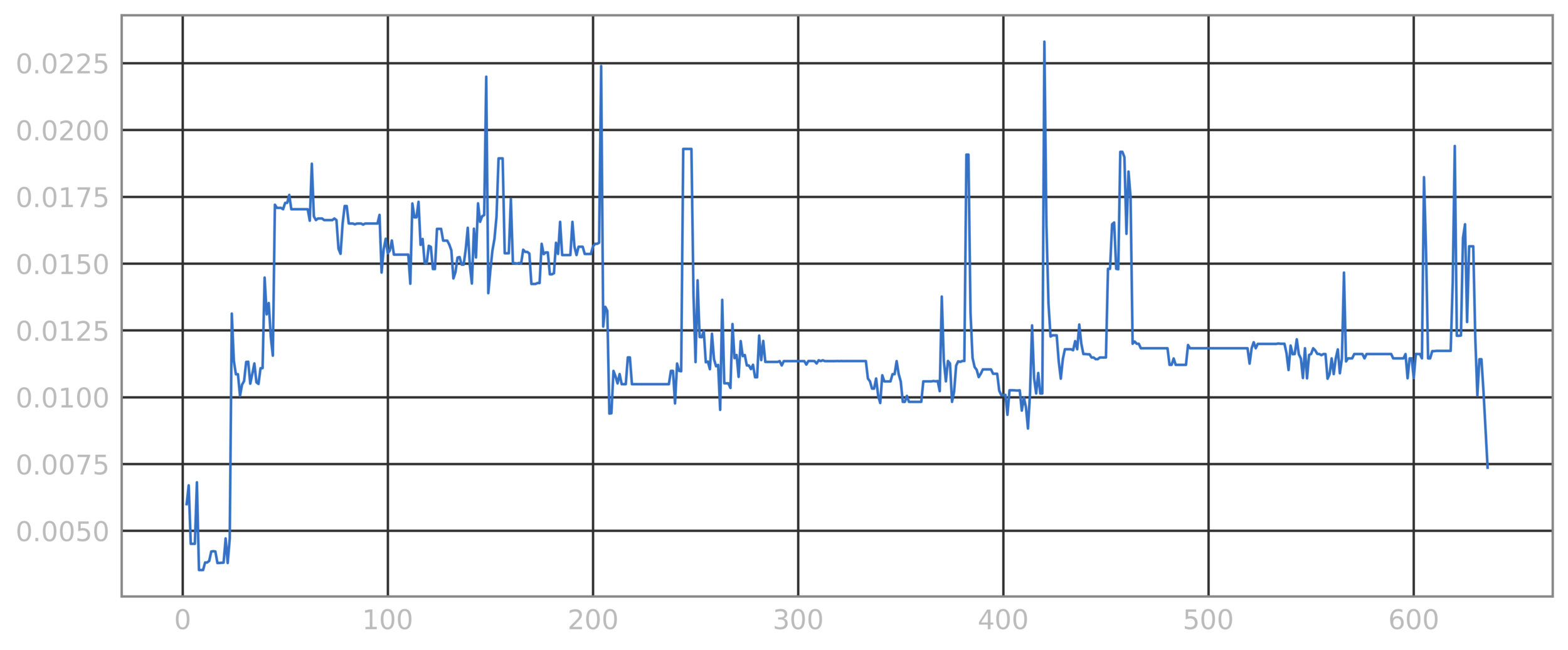
8 75 87 97 141 154 165 178 181 183 203 205 211 216 230 252 327 361 506 588
Local potential fields can be computed given the LSM and dynamical considerations, which reveal future evolution
Stable
(captured by local extrema)
Free to move locally towards extrema
Observation: This lineage (Mississippi lineage) is now extinct since 2022/23
stable lineage
Define Lagrangian\(\dag\)
Over-damped Gradient flow Equation\(\dag\)
where \(-g^{km}\) is the inverse metric tensor
kinetic energy
potential energy
Goldstein, Herbert, et al. Classical Mechanics. 3rd ed., Pearson, 2002.
\(^\dag\)
Principle of stationary action
Local potential field eqn
Stable
(captured by local extrema)
Free to move locally towards extrema
Influenza C : strains and their neighborhoods
Observation: This lineage (Mississippi lineage) is now extinct since 2022/23
stable lineage
Local potential fields can be computed given the LSM and dynamical considerations, which reveal future evolution
By Ishanu Chattopadhyay
DARPA-EA-25-02-05-MAGICS-PA-025


