Generative Models, Drug design and Chemically informed latent spaces
Vidhi Lalchand
13-06-2025

Universitetet i Oslo
Give data samples \( \{x\}_{n=1}^{N}\), learn the probability distribution of data \(p(x)\).
Once you learn \(p(x)\), you can sample from it to generate new instances of the data, \( x_{new} \sim p(x)\).
Data can be high-dimensional, like text, speech, images, molecules.
In a discriminative model, we instead directly learn the conditional distribution \(p(y|x)\) i.e. a decision boundary, in the case of classification, or regression models we learn to predict \( y\) from \( x\).
In the presence of labels \(y\), generative models learn the joint probability distribution of data \(p(x, y)\).
Generative models can also perform discriminative tasks.
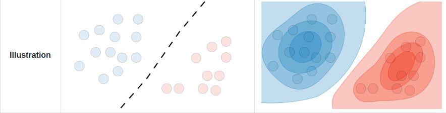
Generative vs. Discriminative Models
|
Smith MJ, Geach JE. Astronomia ex machina: a history, primer and outlook on neural networks in astronomy. Royal Society Open Science. 2023 May 31;10(5):221454.
|
Generative models are powerful tools for embeddings discrete objects into a continuous space, thereby allowing one to simulate them.
Latent space
The Basic Notion of Generative Models
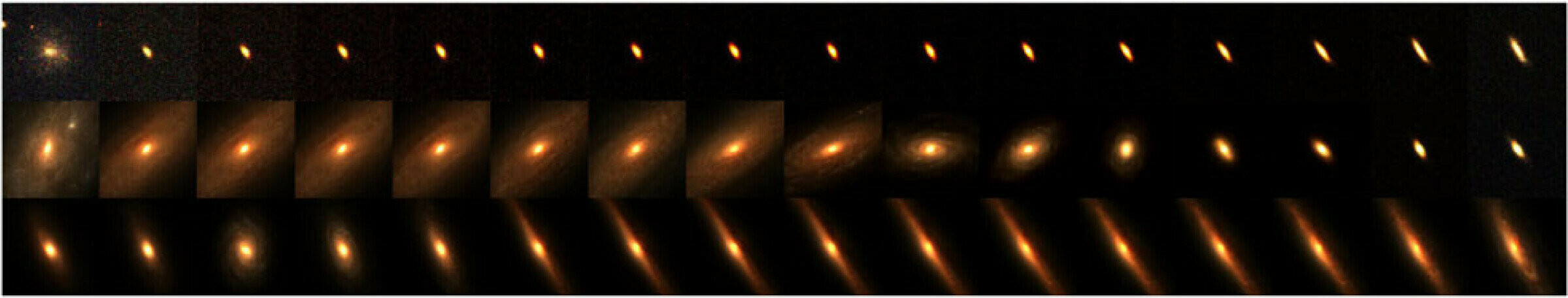
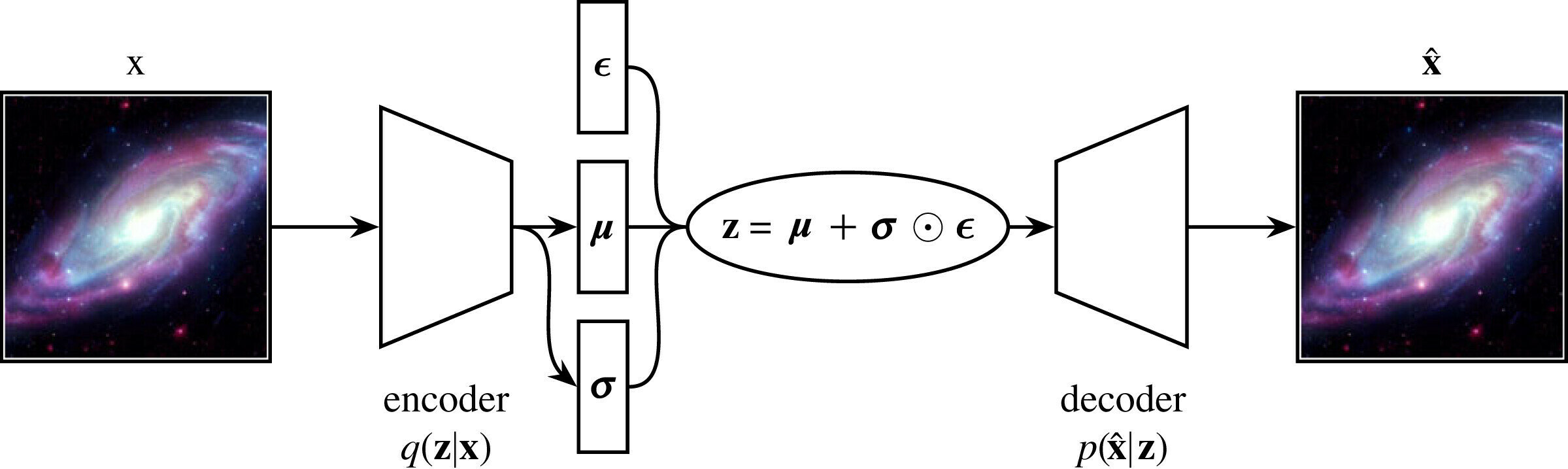
Interpolating between the continuous representation of astronomical objects in latent space
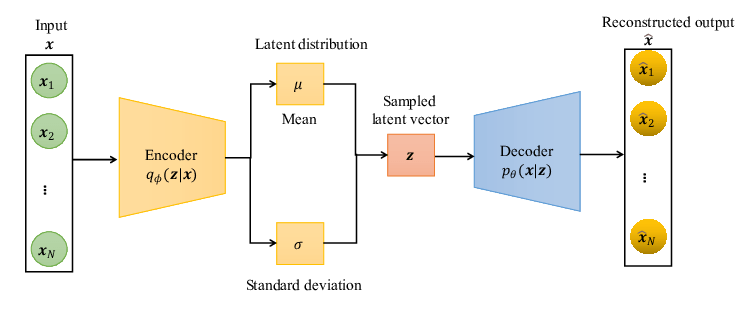
Typical autoencoder style architecture of generative models
Interpolating between the continuous representation of astronomical objects in latent space
Smith MJ, Geach JE. Astronomia ex machina: a history, primer and outlook on neural networks in astronomy. Royal Society Open Science. 2023 May 31;10(5):221454.
Generative Models \( \longrightarrow\) Latent Variable Models
Latent variable models (LVMs) are a powerful class of generative models that introduce hidden (latent) variables to explain observed data.
Let \(z\) denote a 2d latent variable [position, radius]
One can generate \( \mathbf{x}\) given \( \mathbf{z}\), \( \mathbf{z} \longrightarrow \mathbf{x}\).
The structure of the data is captured by the compressed latent variable \(\mathbf{z}\), while the data representation in pixels is several hundred dimensions.
\( \mathbf{x}\)
In real data, \( \mathbf{z}\) is not explicitly known, it has to be learnt from the data.
The fundamental assumption underlying LVMs is that the data generation process involves some latent variable \( \mathbf{z}\). The data \(\mathbf{x}\) is generated through \(\mathbf{z}\).
\( \mathbf{x}\)
\( \mathbf{z}\)
Inference \( q_{\phi}(\mathbf{z}|\mathbf{x})\)
Generation \( p_{\theta}(\mathbf{x}|\mathbf{z})\)
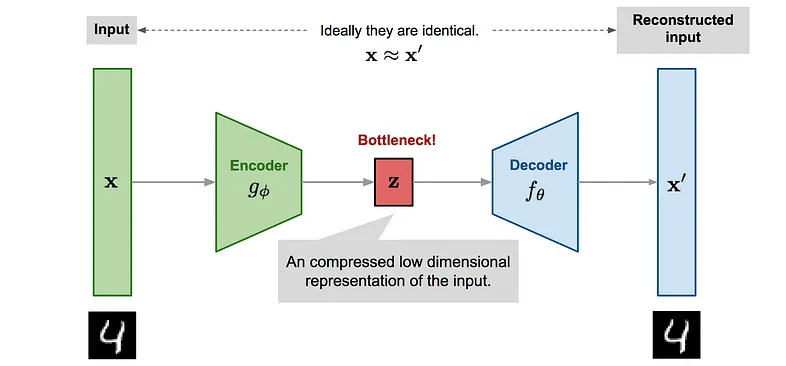
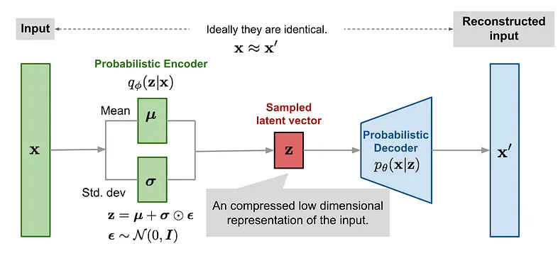
Autoencoders \( \longrightarrow\) Variational AEs
Reconstructed input
In VAEs we want to maximise the ELBO so the loss function is negative of the ELBO.
The reconstruction likelihood encourages the decoder to accurately reconstruct the data from the latent \(\mathbf{z}\).
The KL term forces points to stay close to the prior, exerting a counter weight.
The reconstruction likelihood encourages the decoder to accurately reconstruct the data from the latent \(\mathbf{z}\).
Autoencoders v. Variational AEs
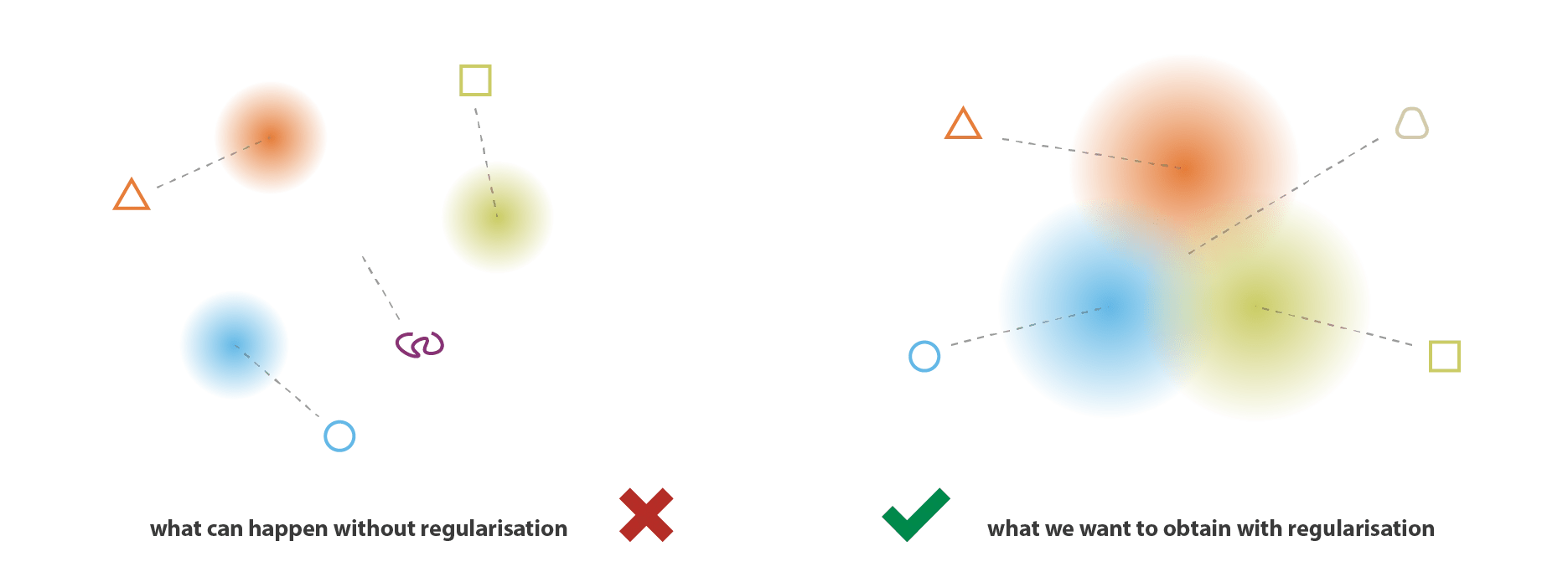
VAEs can be viewed as a "regularised" version of an autoencoder. It is trained to preserve two properties of the latent space:
1. Continuity
2d \(\mathbf{z}\) space
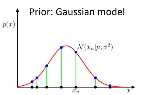
Prior \(p(\mathbf{z}) = \mathcal{N}(0,1)\)
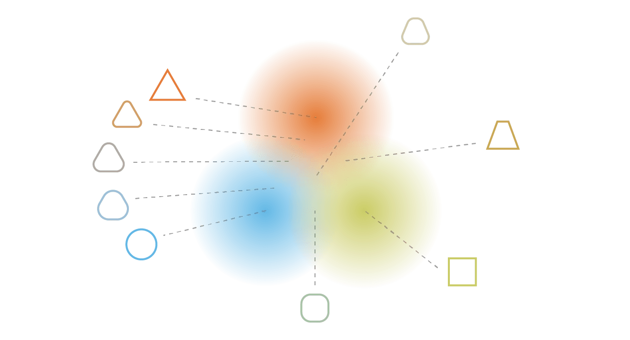
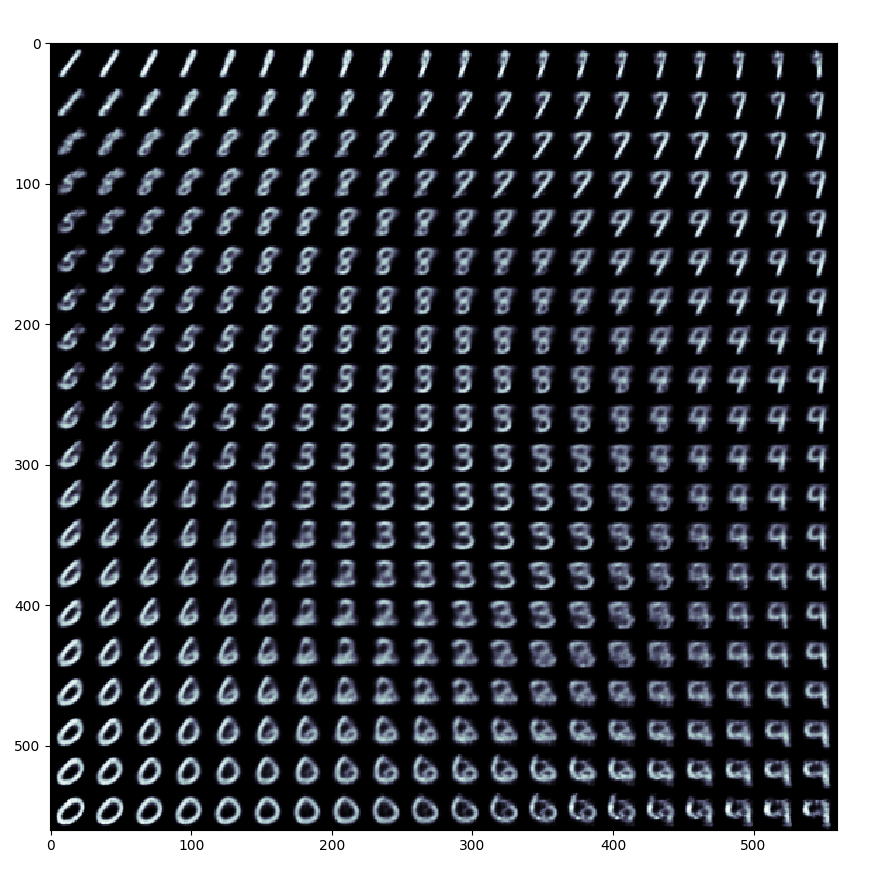
Smooth transitions in latent space should correspond to smooth transitions in data space.
Points in an epsilon-neighbourhood of a reference point should have very similar outputs.
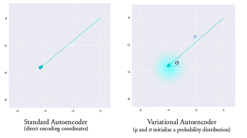
A single encoding of an autoencoder vs. a variational autoencoder in a 2d latent space.
The entire latent space in a VAE comprises these soft ellipsoidal regions denoting Gaussian distributions.
2. Completeness
Sampling randomly from the prior should lead to plausible data instances.
2d \(\mathbf{z}\) space
Autoencoders v. Variational AEs
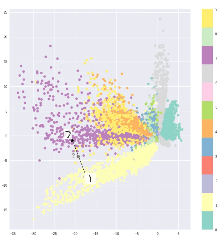
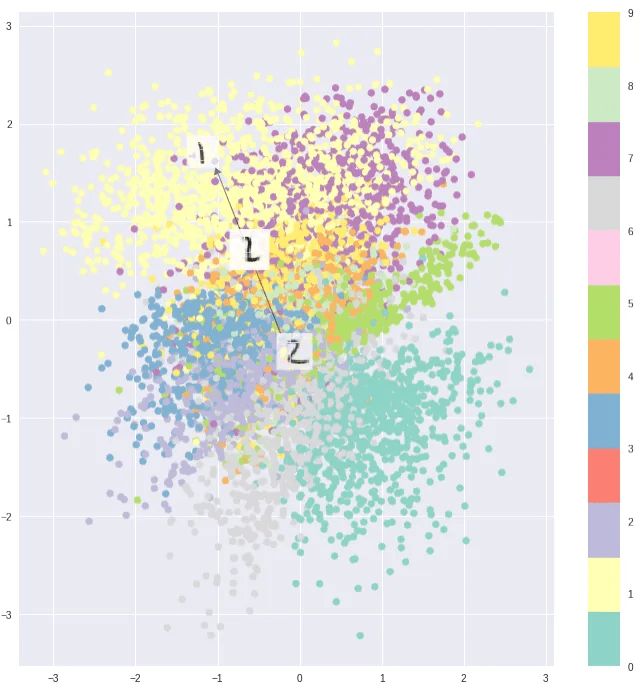
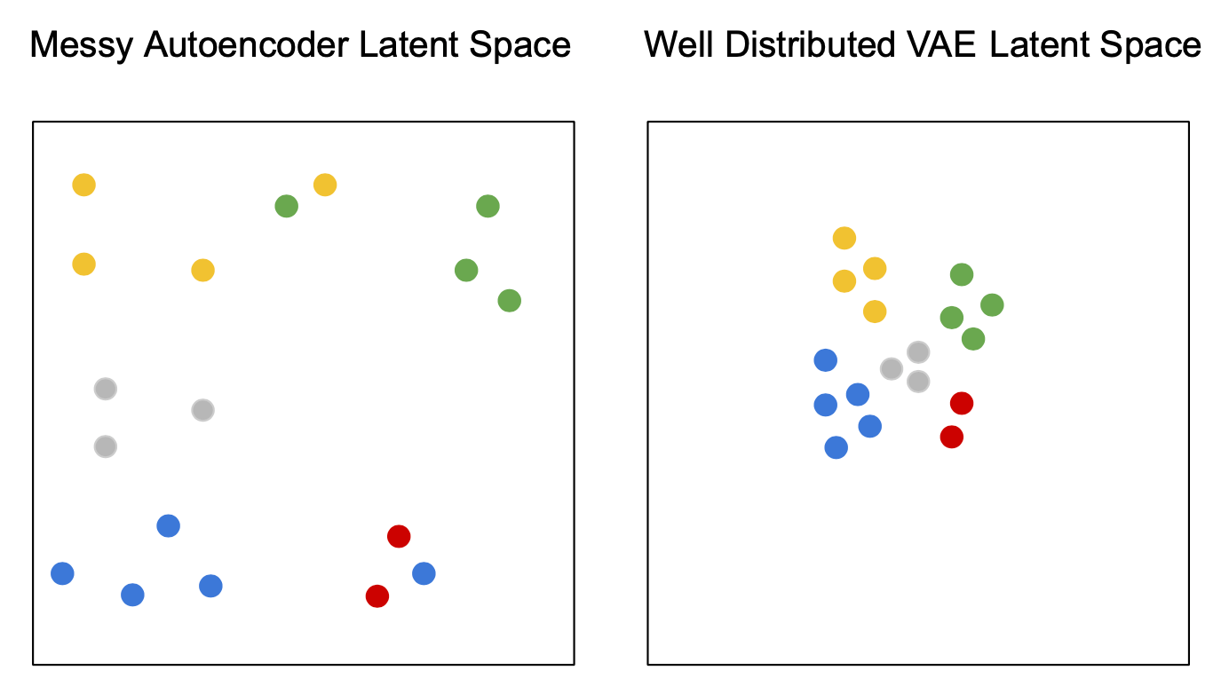
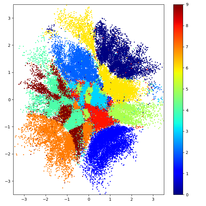
Visualization of the 2d latent space of an AE and a VAE trained on MNIST data, data dim = 28 x 28, latent dim = 2
In contrast to the autoencoder latent space the clusters are densely packed close to the prior permitting sensible interpolation.
The latent space shows the cluster-forming nature of the encodings encouraged by the reconstruction loss objective. Distinct encodings for each image type makes it easier for the decoder to decode them, but the space is non-contiguous.
AE
VAE
VAEs & Posterior Collapse
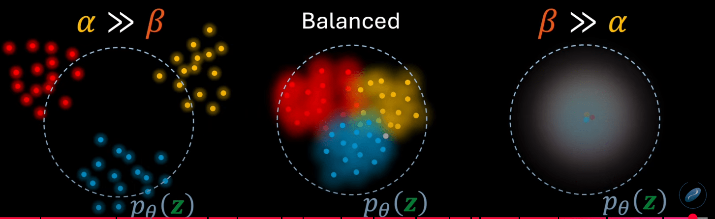
VAE Loss = \( \mathcal{L}_{\text{recon}} + \mathcal{L}_{\text{KL}}\)
The VAE loss has to strike a delicate balance between reconstruction and regularisation.
~Autoencoder
Posterior collapse
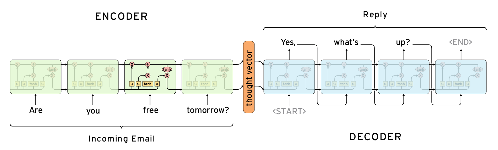
Autoregressive decoders (with/without a latent space)
In language Seq2Seq models it is quite standard to remove latent variables all together and just have a single deterministic context vector.
Such models are typically used for question answering, machine translation. The encoder is always used together with the decoder, at inference time.
Several important use cases in biomedical applications involve operating and navigating the latent space. Post training we need to be able to go from an arbitrary point in latent space to data, via the decoder.
Navigating chemical space with latent flows.
Latent-based Directed Evolution accelerated by Gradient Ascent for Protein Sequence Design
Low-dimensional learnt feature spaces for vocal context repositories
- GPs can be used in the unsupervised settings by learning a non-linear, probabilistic mapping from latent space \( \mathbf{X} \) to data-space \( \mathbf{Y} \).
- We assume the inputs \( \mathbf{X} \) are latent (unobserved).
Given: High dimensional training data \( \mathbf{Y} \equiv \{\bm{y}_{n}\}_{n=1}^{N}, Y \in \mathbb{R}^{N \times D}\)
Learn: Low dimensional latent space \( \mathbf{X} \equiv \{\bm{x}_{n}\}_{n=1}^{N}, X \in \mathbb{R}^{N \times Q}\)
Lalchand et al. (2022)
Gaussian Processes for Latent Variable Modelling (at scale)
Vidhi Lalchand, Aditya Ravuri, Neil D. Lawrence. Generalised GPLVM with Stochastic Variational Inference. In International Conference on Artificial Intelligence and Statistics (AISTATS), 2022
The GPLVM is probabilistic kernel PCA with a non-linear mapping from a low-dimensional latent space \( \mathbf{X}\) to a high-dimensional data space \(\mathbf{Y}\).
The Gaussian process mapping
High-dimensional data space
. . .
. . .
N
D
\( X \in \mathbb{R}^{N \times Q}\)
\( f_{d} \sim \mathcal{GP}(0,k_{\theta})\)
\( Y \in \mathbb{R}^{N \times D} (= F + noise)\)
Robust to missing dimensions in training data (missing at random)

Vidhi Lalchand, Aditya Ravuri, Neil D. Lawrence. Generalised GPLVM with Stochastic Variational Inference. In International Conference on Artificial Intelligence and Statistics (AISTATS), 2022
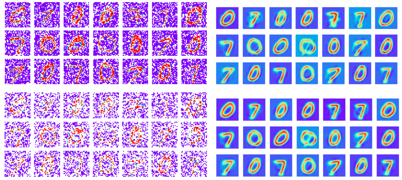
30%
60%
Training data: MNIST images with masked pixels
Reconstruction
Note: This is different to tasks where missing data is only introduced at test time
Learning to reconstruct dynamical data
Autoregressive Generative Models are a paradigm of choice for search and design of new drugs.
It's a widely cited estimate that there are around 106010^{6010
1010010^{100}~\(10^{60}\) chemically valid, synthetically accessible small molecules, even under fairly conservative definitions of "small."
Why is drug-design an interesting problem in the first place?
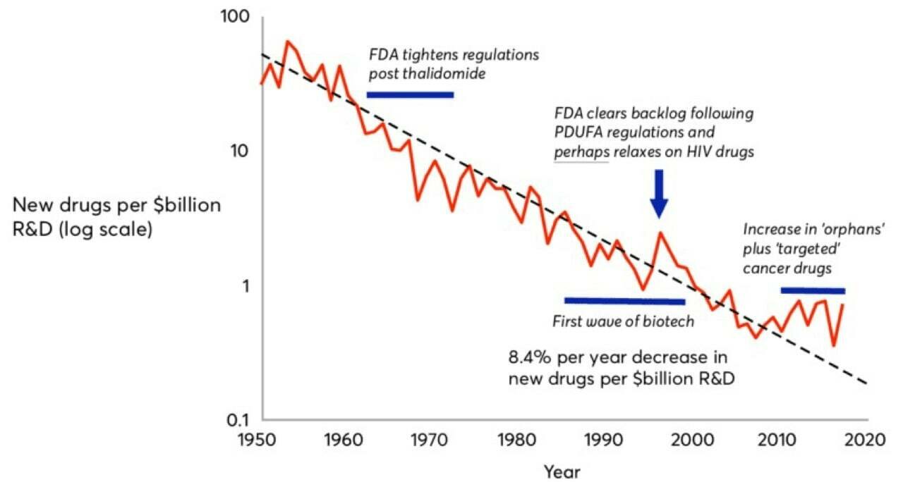
Drug discovery has been witnessing an inverse of Moore's law -- pharma companies are spending increasingly more $ on fewer drugs (drugs brought to market per billion$ of R&D).
Eroom's law!
Roadmap: Unlocking machine learning for drug discovery. Bessember Venture Partners Technical Report, 2021.
Virtual screening or De novo molecular design
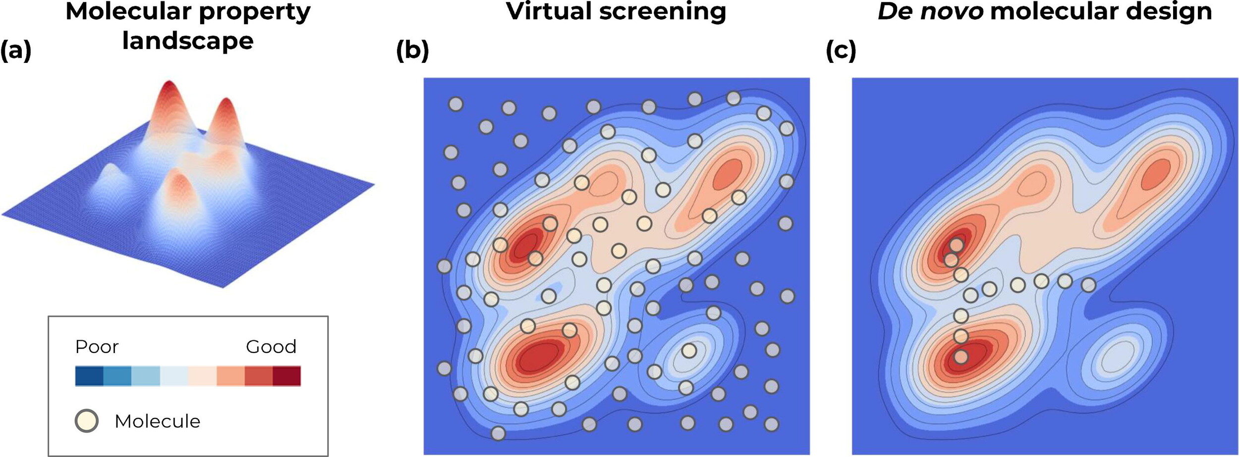
Screen from a finite list of known molecules
Traverse the continuous representation of the chemical space (through optimisation)
Generative approaches for de novo molecular design
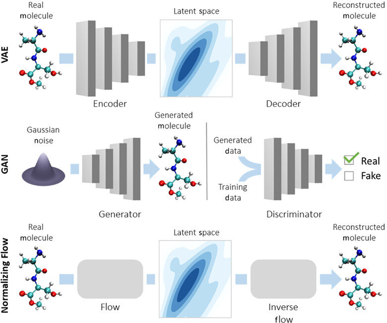
Gómez-Bombarelli R, et al. Automatic chemical design using a data-driven continuous representation of molecules. ACS central science. 2018. (ChemicalVAE)
Kusner MJ et al. Grammar variational autoencoder. InInternational conference on machine learning, 2017. (GrammarVAE)
Jin W et al. Junction tree variational autoencoder for molecular graph generation. InInternational conference on machine learning 2018. (JT-VAE)
De Cao N, Kipf T. MolGAN: An implicit generative model for small molecular graphs. ICML Workshop for Applications of Deep Generative Models. 2018. (MolGAN)
Kang S, Cho K. Conditional molecular design with deep generative models. Journal of chemical information and modeling. 2018. (SSVAE)
Zang C, Wang F. Moflow: an invertible flow model for generating molecular graphs. InProceedings of the 26th ACM SIGKDD international conference on knowledge discovery & data mining 2020. (MoFlow)
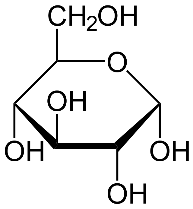
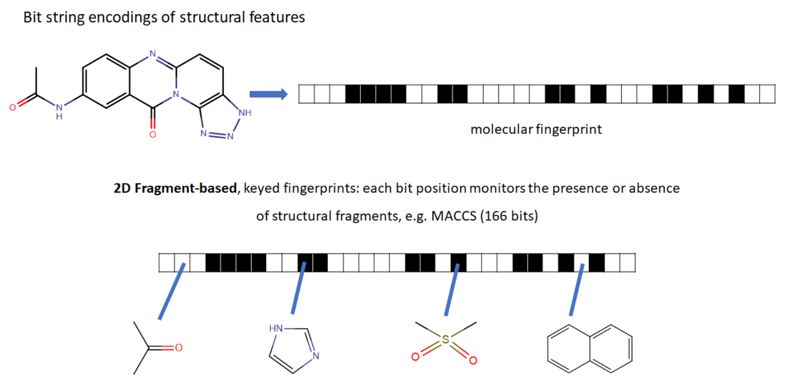
Representation of small drug-like molecules
Understanding how to best represent molecules in a machine-readable format is a key challenge and an active area of research.
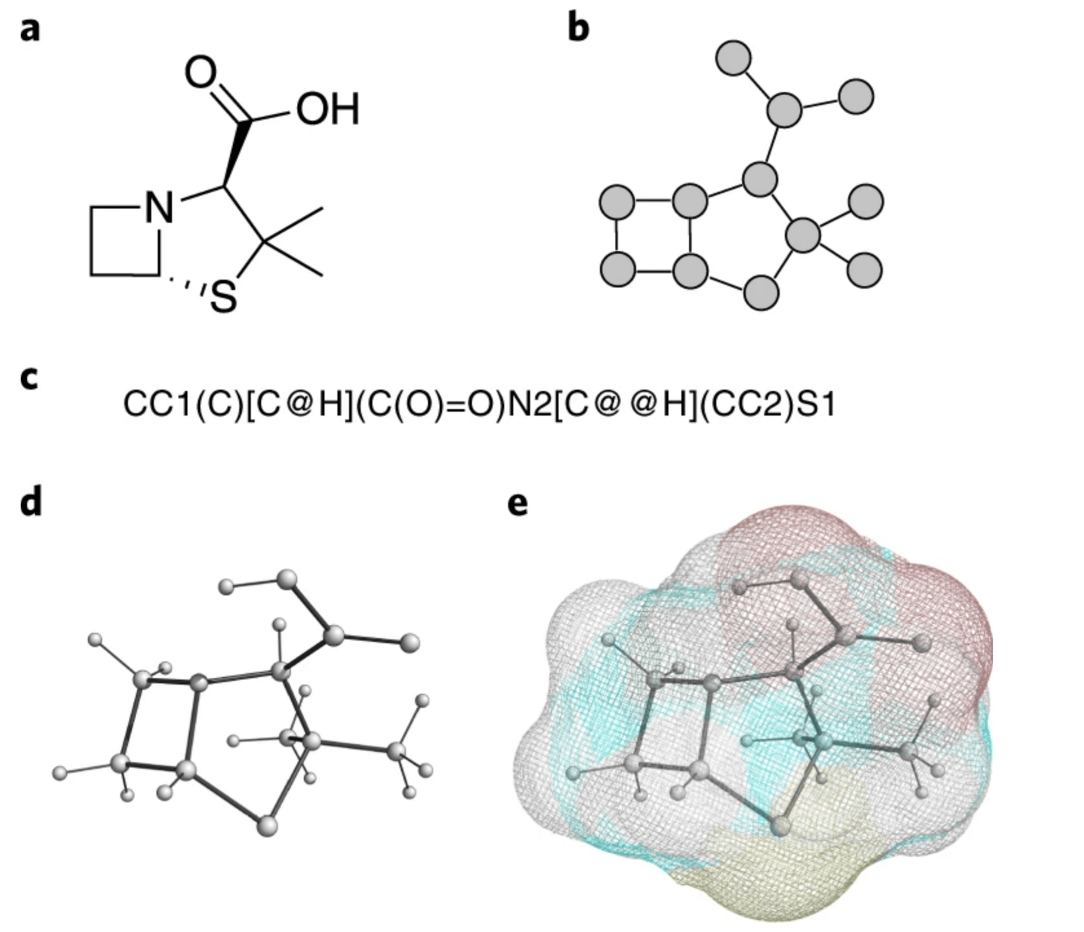
Formally, there are 4 representations which are prevelant in literature:
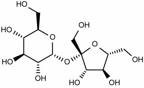
SMILES (Simplified molecular-input line-entry system) is a formalism to generate a string identifier for chemical compounds. It has an alpha-numeric nomenclature which uses atomic letters to denote atoms, parenthesis () to denote branches and symbols =, #,$ to denote double, triple and quadruple bonds.
ECFP (Extended connectivity fingerprints)
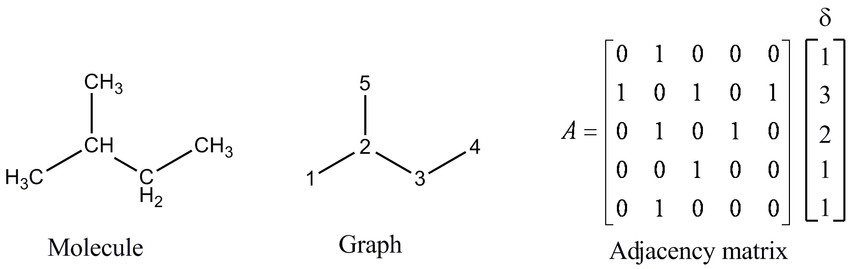
2D graph
3D graph
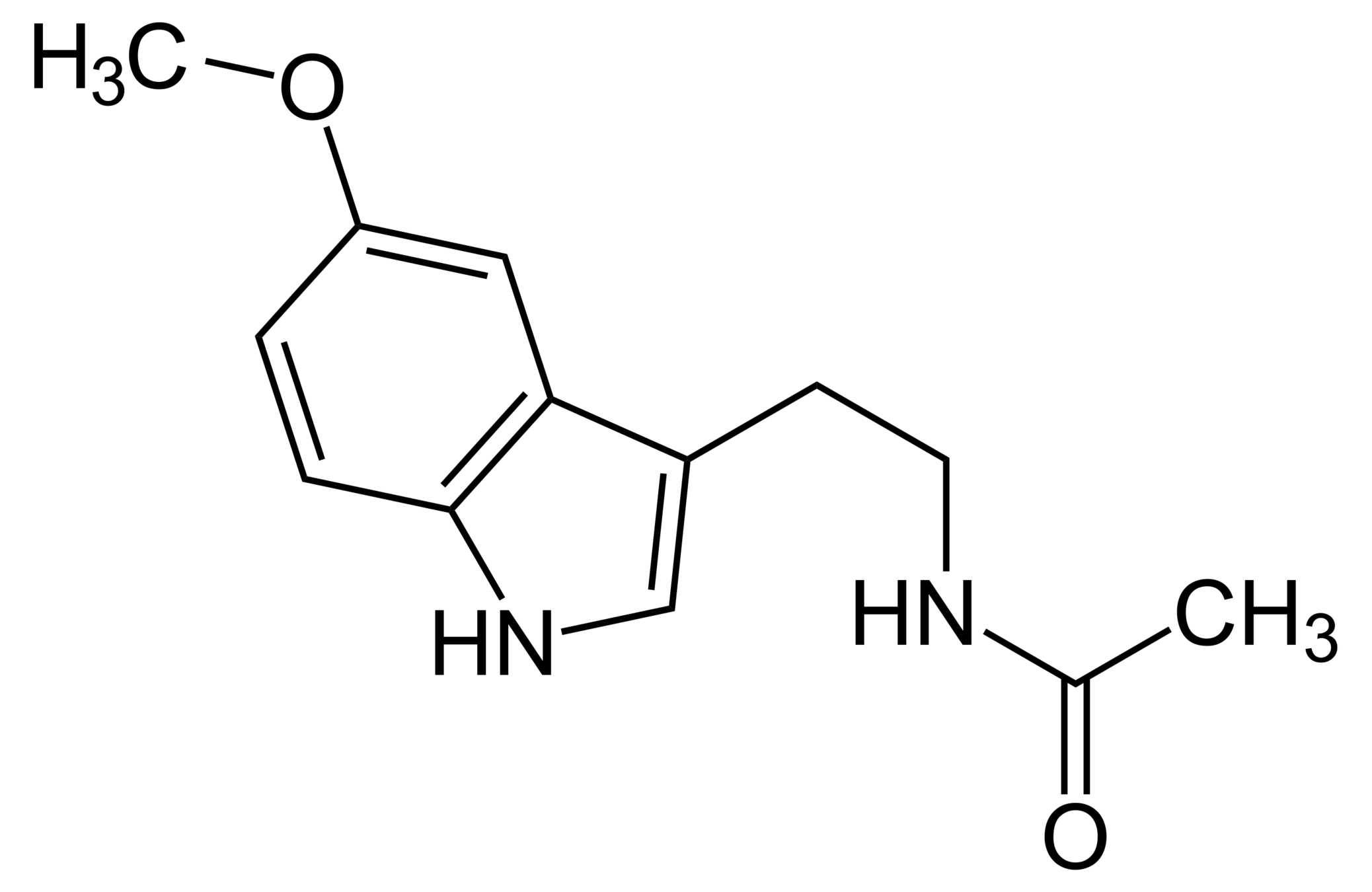

CC(=O)NCCC1=CNc2c1cc(OC)cc2
CN1CCC[C@H]1c2cccnc2
Melatonin
Nicotine
The problem with SMILES
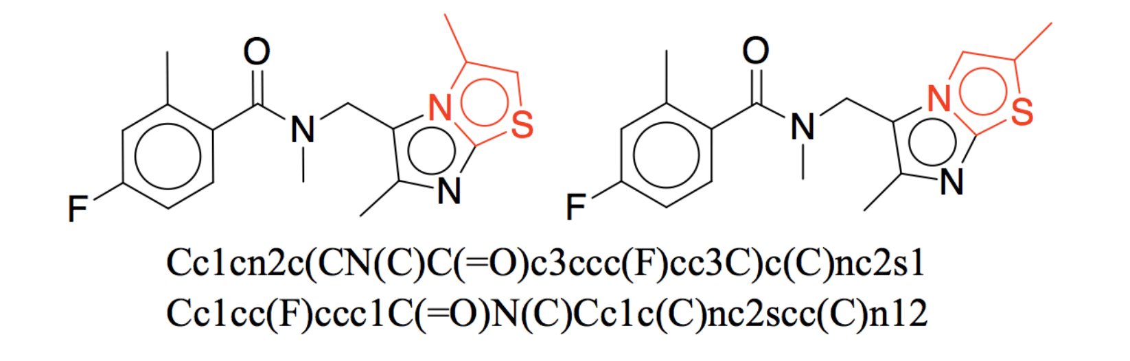
Two almost identical structures with very different SMILES strings.
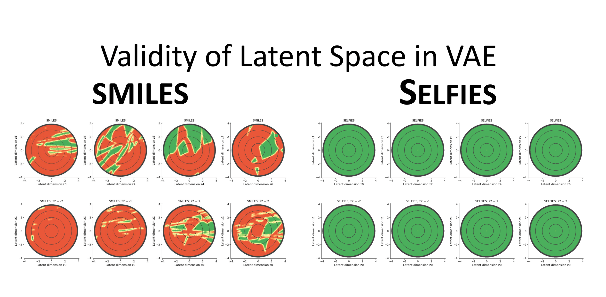
Red denotes dead regions in the latent space which decode to invalid strings.
Jin W, Barzilay R, Jaakkola T. Junction tree variational autoencoder for molecular graph generation. InInternational conference on machine learning 2018 Jul 3 (pp. 2323-2332). PMLR.
Krenn M, Häse F, Nigam A, Friederich P, Aspuru-Guzik A. Self-referencing embedded strings (SELFIES): A 100% robust molecular string representation. Machine Learning: Science and Technology. 2020 Oct 28;1(4):045024.
SELFIES: A robust molecular representation
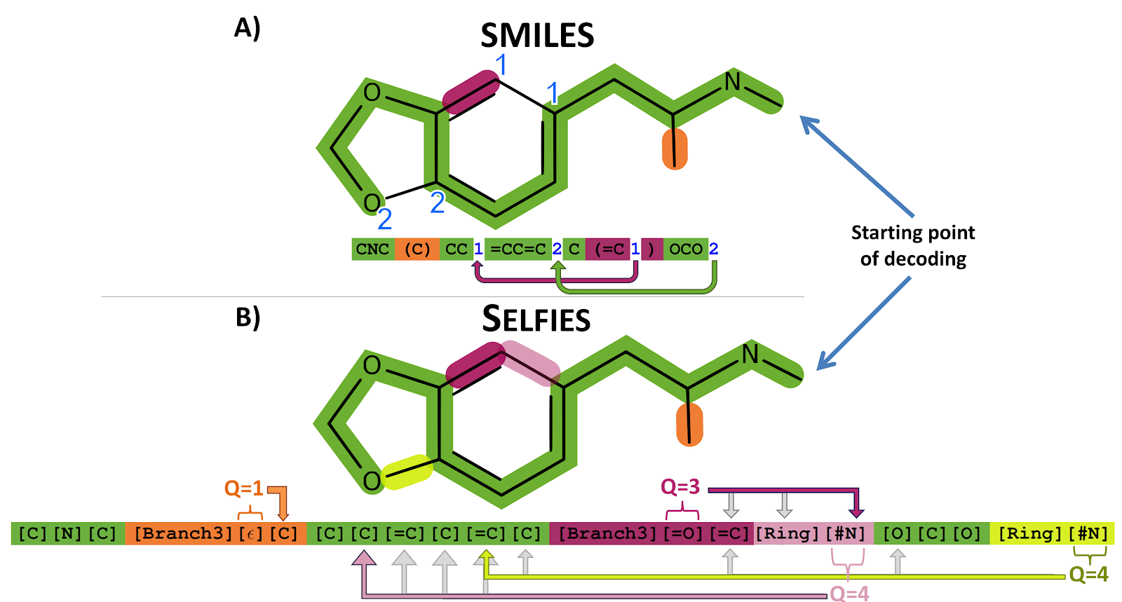
Every SELFIES string constructed from its alphabet corresponds to a valid chemical graph.
Self-referencing embedded strings (SELFIES) are built upon ‘semantically constrained graphs’ so that each symbol in the string can be used to convert it into a unique graph.
Krenn M, Häse F, Nigam A, Friederich P, Aspuru-Guzik A. Self-referencing embedded strings (SELFIES): A 100% robust molecular string representation. Machine Learning: Science and Technology. 2020 Oct 28;1(4):045024.

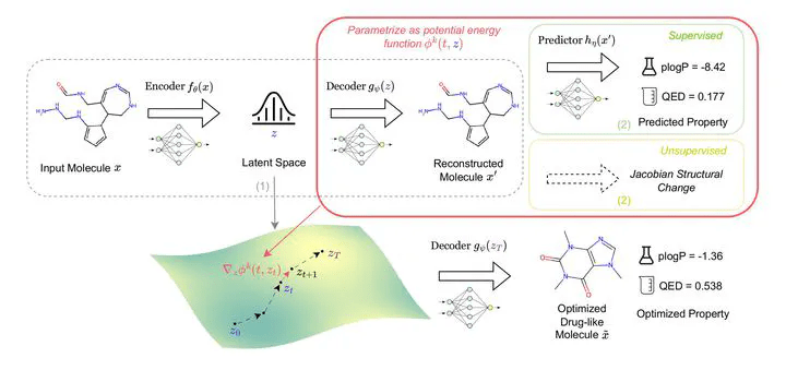
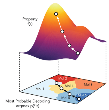
Generative model + Property prediction
How do we use generative modelling to identify molecules which optimise a property of interest?
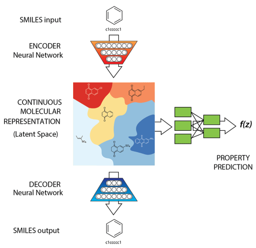
Gómez-Bombarelli R, et al. Automatic chemical design using a data-driven continuous representation of molecules. ACS central science. 2018. (ChemicalVAE)
Goal: Propose a generative model which worked on SELFIES string representation of molecules and additionally, regularise the latent space as a function of properties of interest.
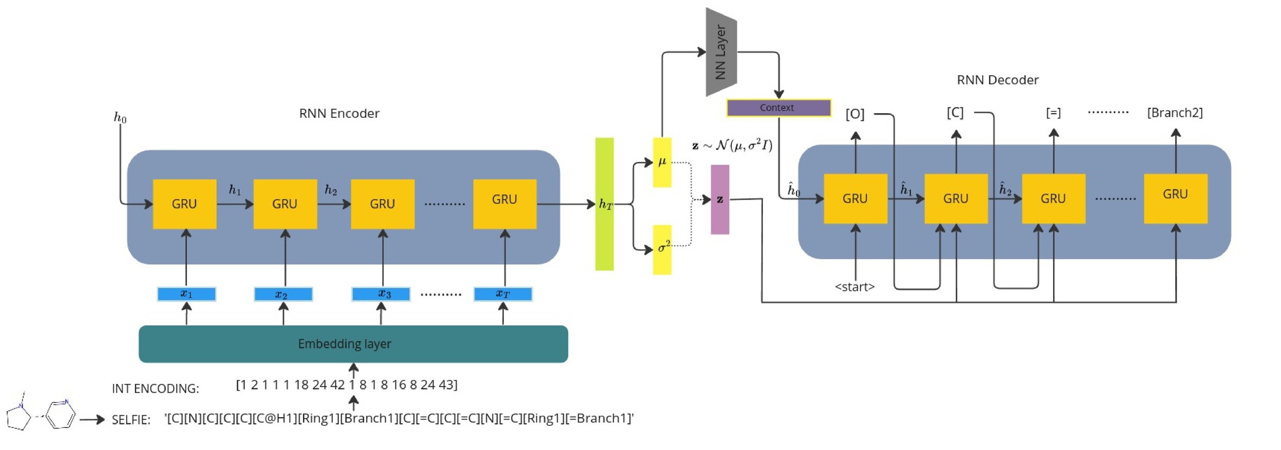
Seq2Seq Model with learnt context vector
The latent vector acts as a "bottleneck".
Encoder outputs a context vector and the dynamics between the context and latent have to be carefully controlled.
We wish to do sampling/generation post training, how to initialise the decoder hidden state?
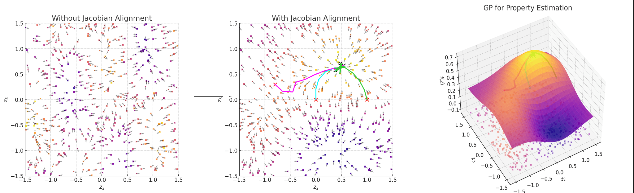
Regularise the seq2seq model with Gaussian process property decoders
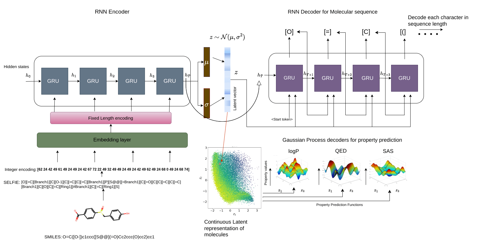
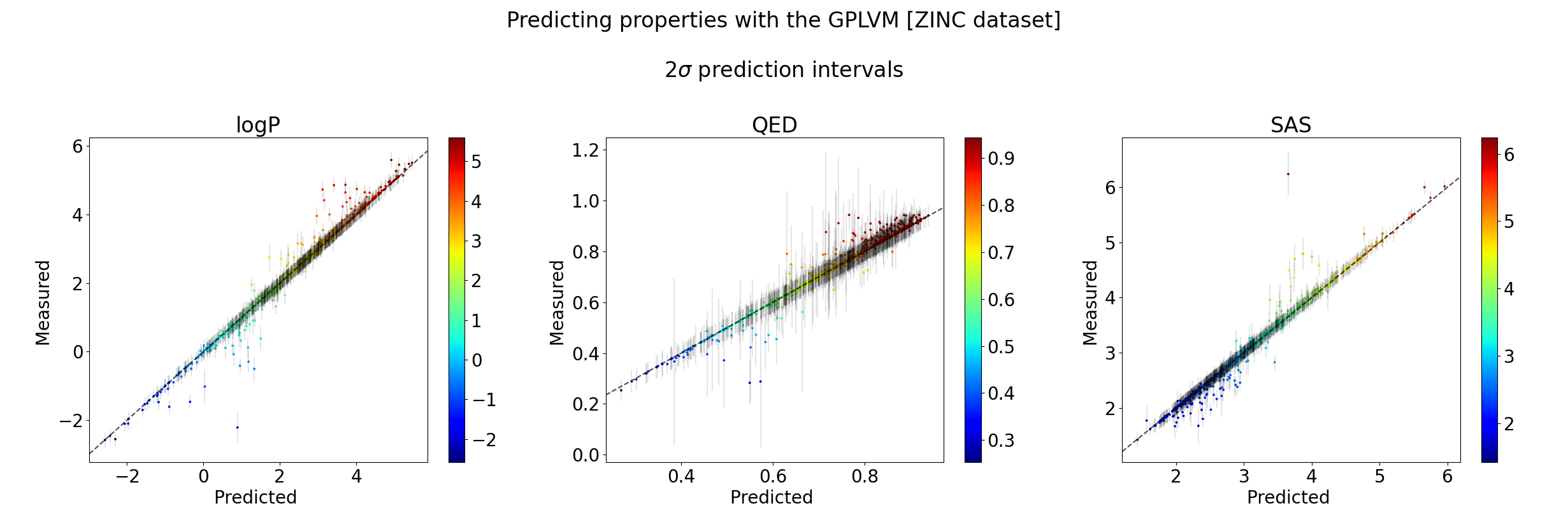
Train Gaussian process mappings from the high-dimensional latent space to scalar properties.
\(\mathbf{y}_{i} = f_{i}(z) + \epsilon, \epsilon \sim \mathcal{N}(0,\sigma^{2})\) [property \(i\)]
\(f_{i} \sim \mathcal{GP}(0, k_{i}(z,z^{\prime}))\)
Smoothness properties of this mapping is controlled by the kernel function \(k_{i}\)
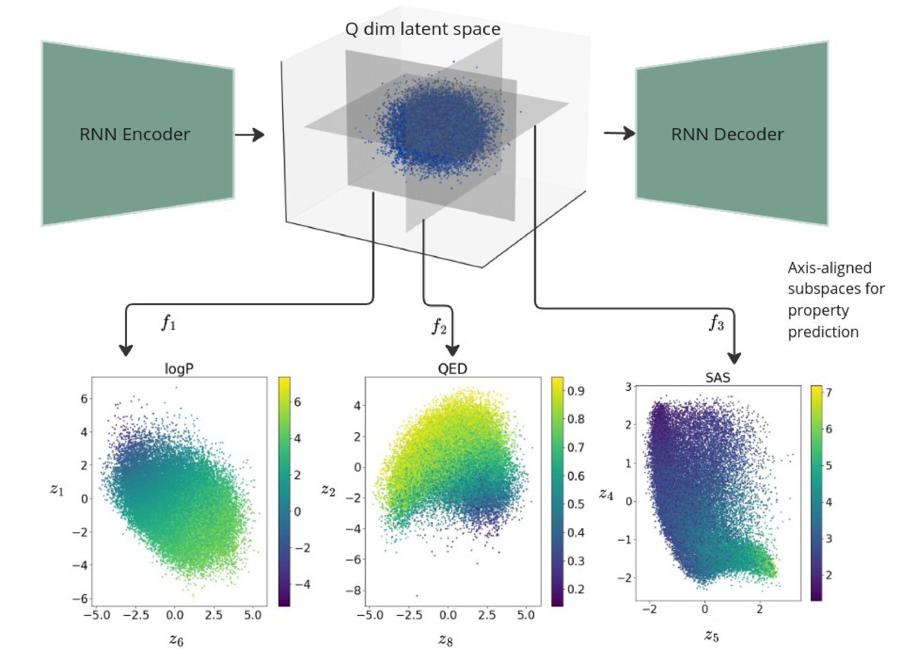
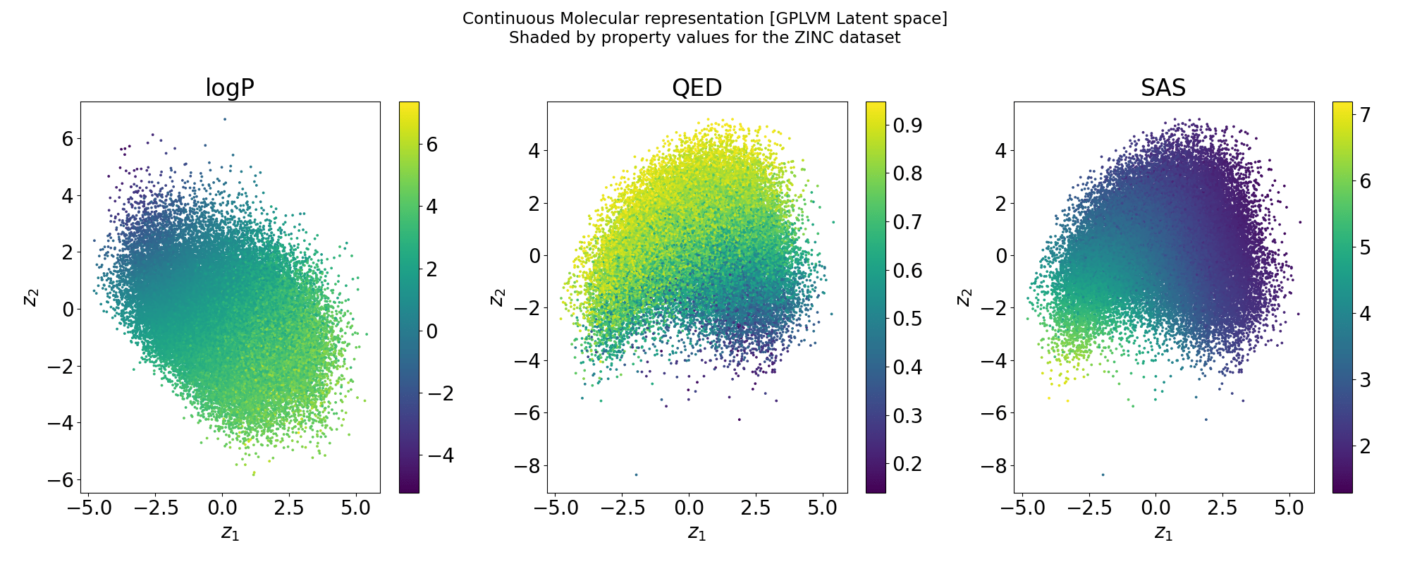
Gaussian process property decoders on the generative latent space
Recurrent VAE + Gaussian process decoders
Overall loss =
Q is the dimensionality of the latent space. The learnt lengthscales in each dimension indicate the influence of that dimension on the prediction.
Joint Model
Seq2Seq Model with SELFIES: Gaussian process property decoders
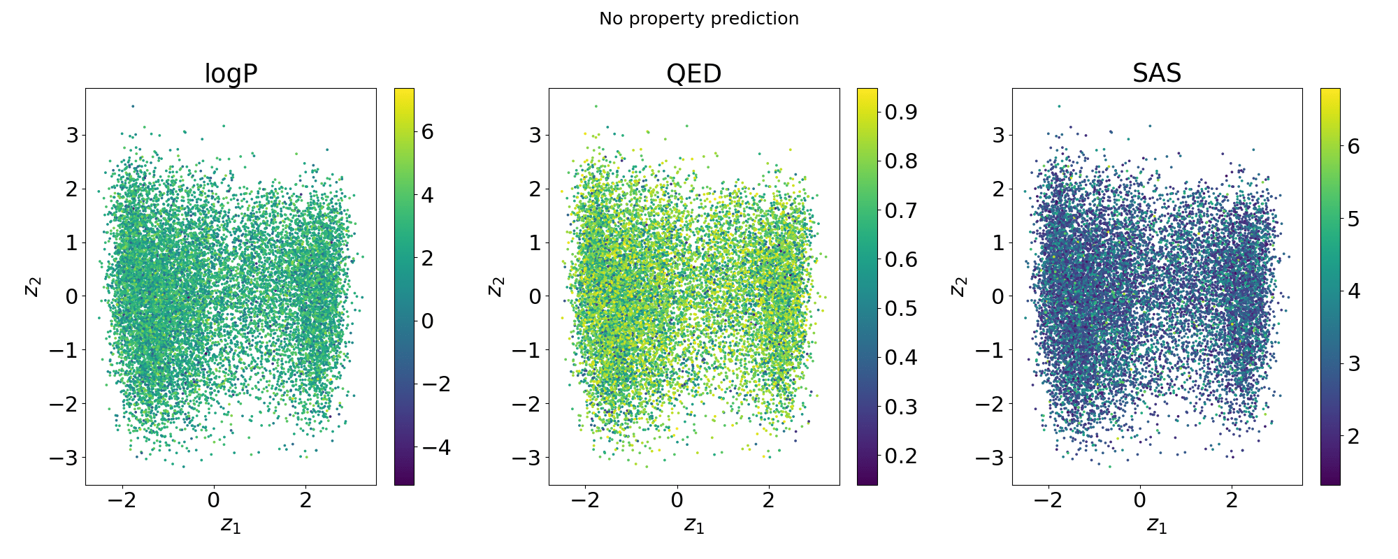
Evaluation criteria & Property prediction
| Size | Recon | Validity | Novelty | |
|---|---|---|---|---|
| QM9 | 66k | 98.2% | 100% | 100% |
| ZINC | 240k | 99.4% | 100% | 100% |
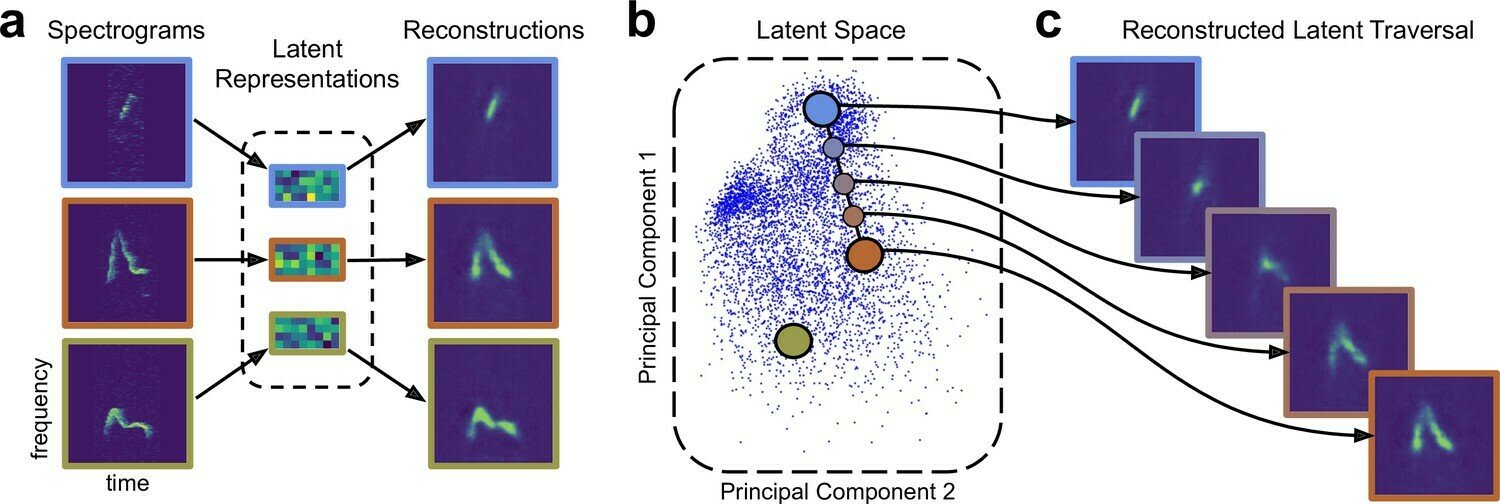
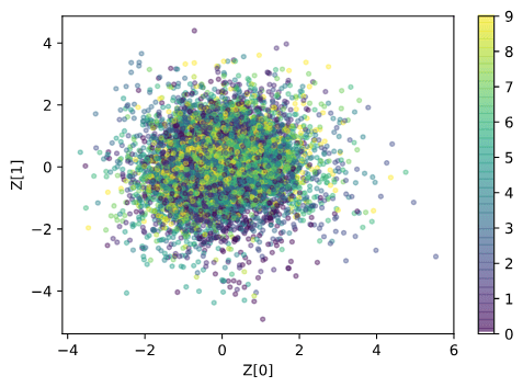
Structure of the latent space: Neighbourhood visualisation
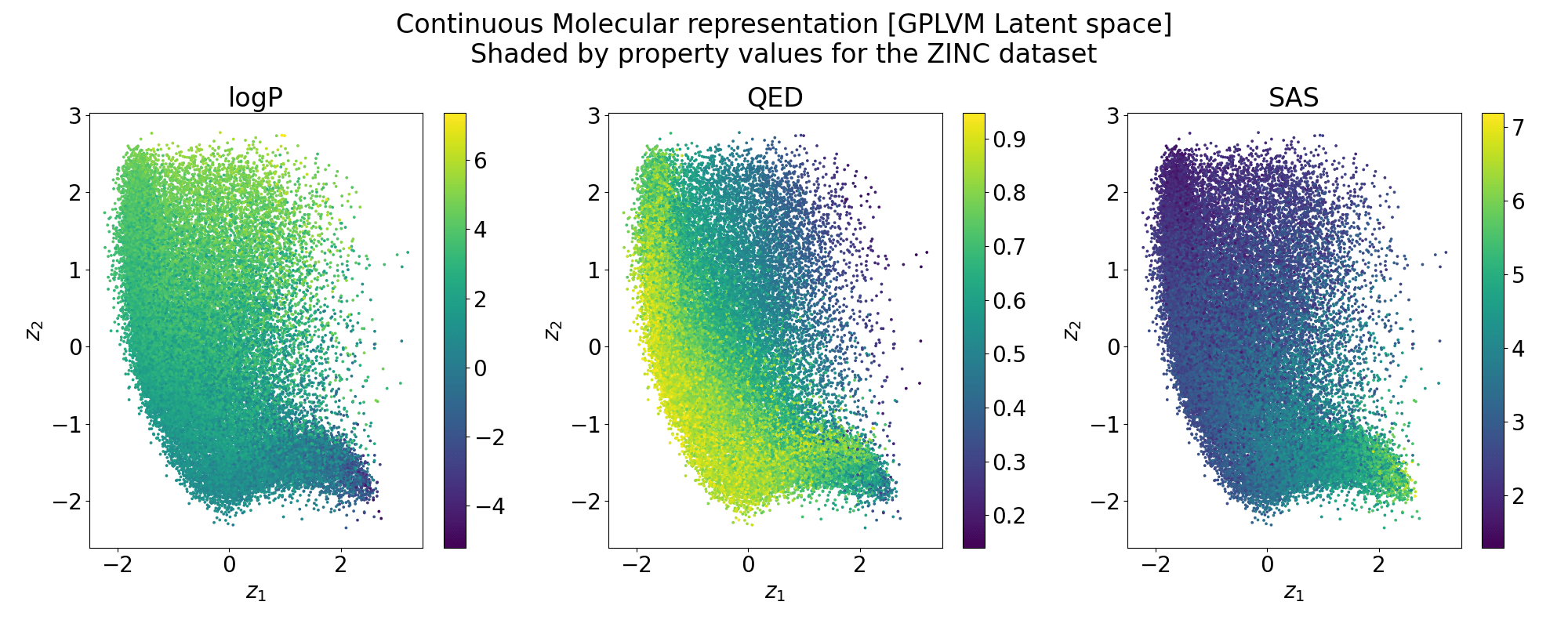
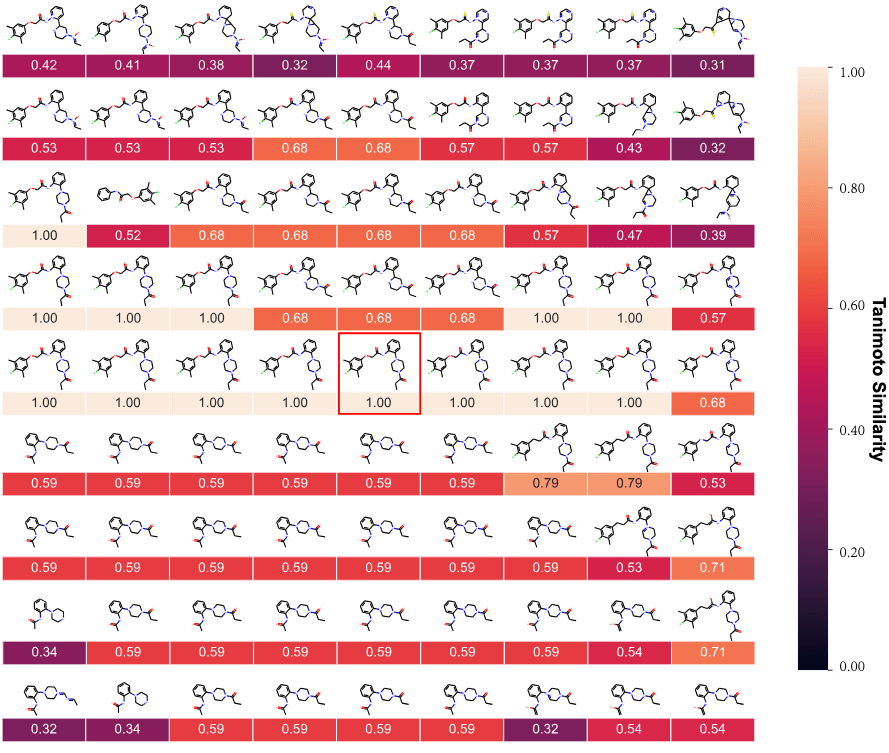
If the latent space is smooth in structure then molecules close in latent space should be close in data space.
Zang C, Wang F. Moflow: an invertible flow model for generating molecular graphs. InProceedings of the 26th ACM SIGKDD international conference on knowledge discovery & data mining 2020 Aug 23 (pp. 617-626)
Traversal over a convex subspace of the latent space
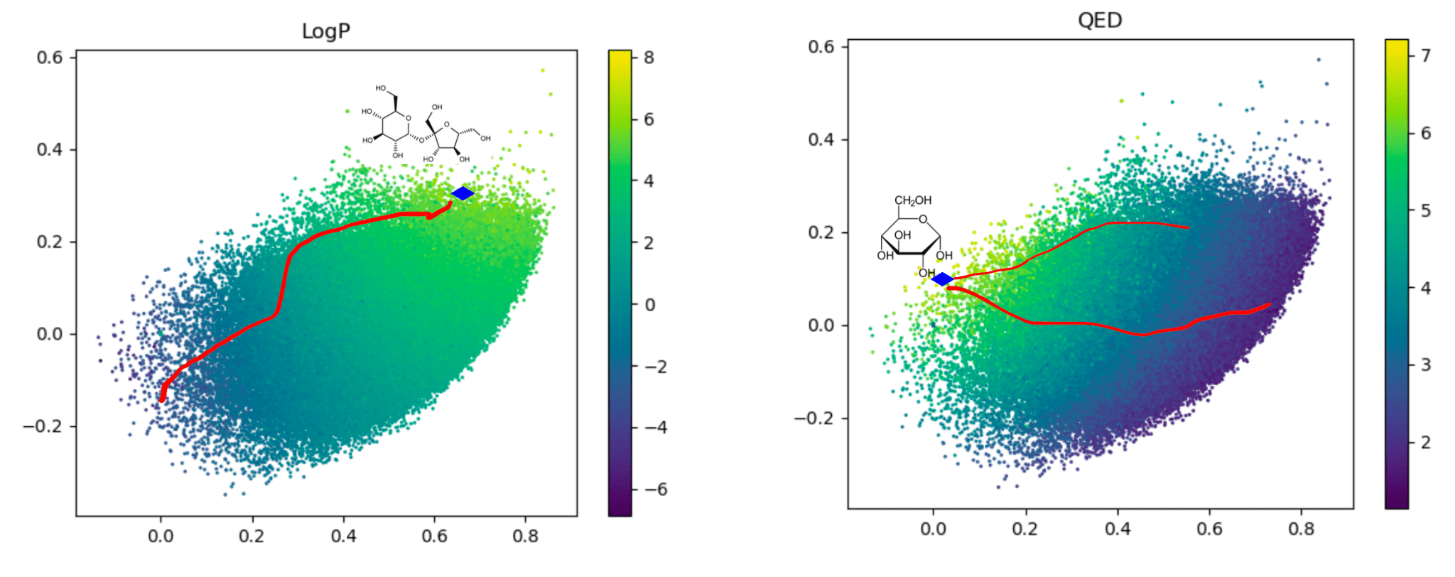
Evolution of a 2d subspace of the latent space during training
Points shaded by actual QED (drug-likeness) scores
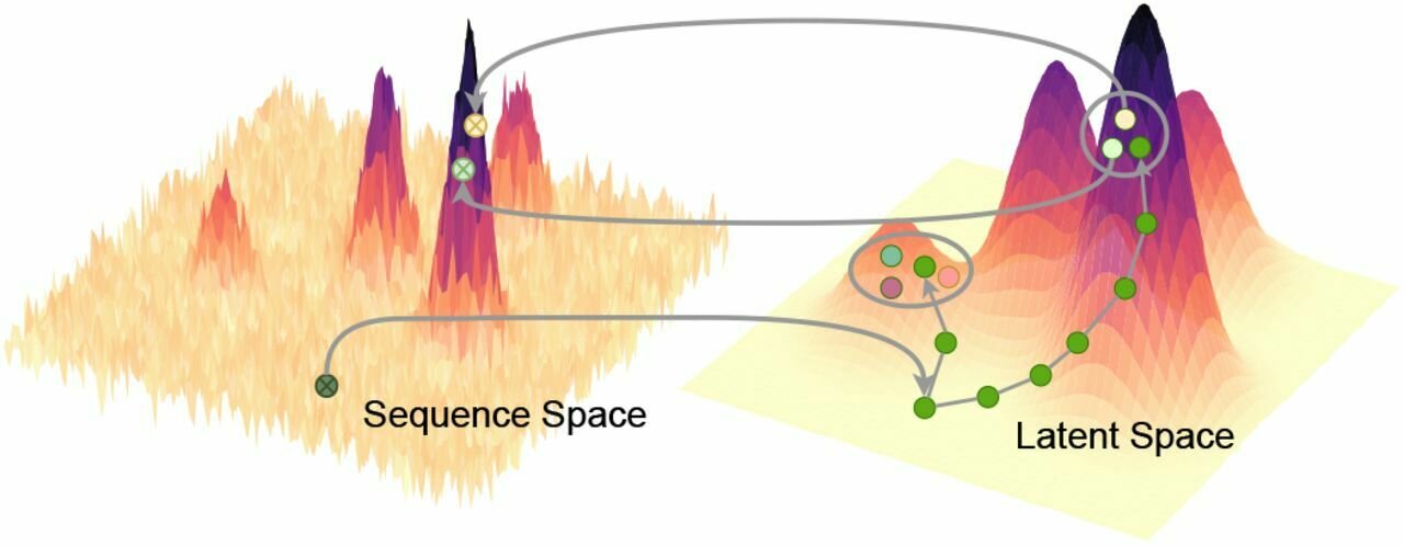
Gaussian Annulus theorem
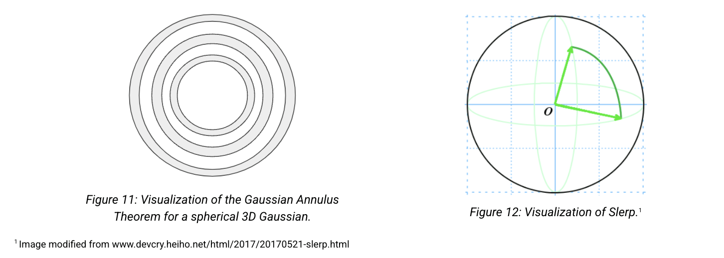
The Gaussian Annulus Theorem tells us that most of the probability mass of a high-dimensional Gaussian lies in a thin shell -- also called, the "soap bubble" effect.
Instead of interpolating between two points by traversing the low-density Euclidean interpolation, traverse across the surface of this high-density shell. This is known as Spherical Linear Interpolation (Slerp).
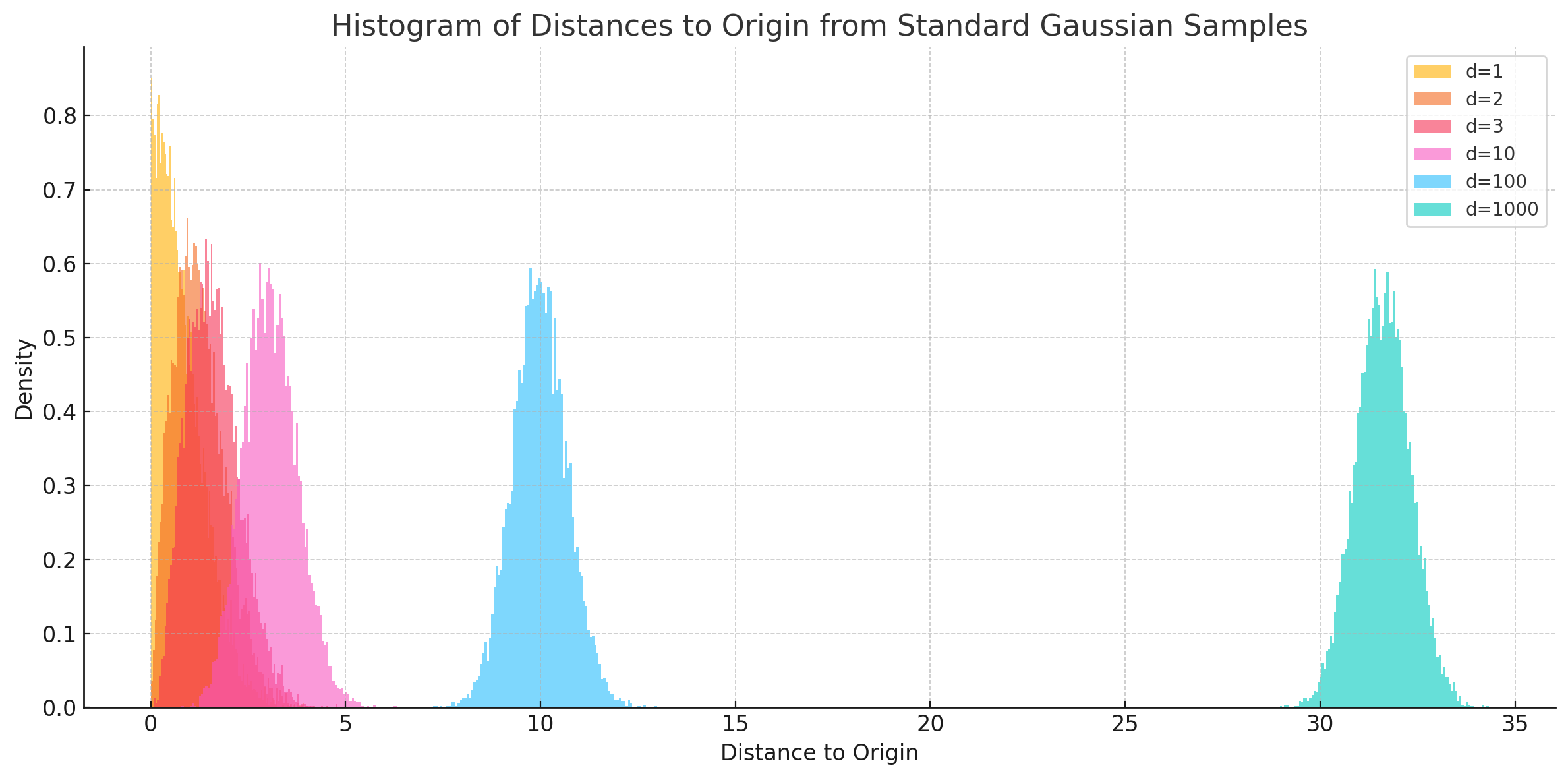
As, \(d \longrightarrow \infty\), the samples pile up almost equidistant from the origin, giving the shell effect.
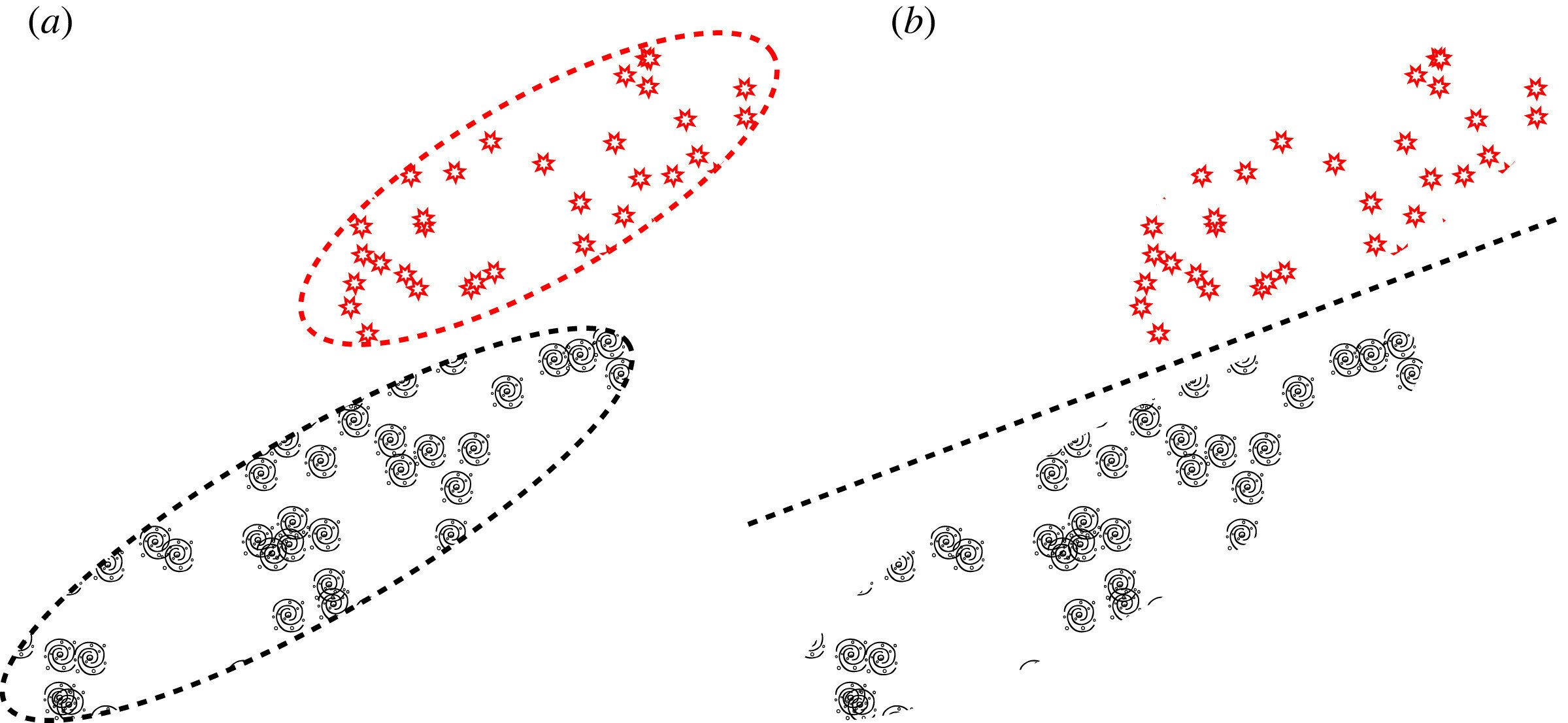
Dead-zones in latent traversals
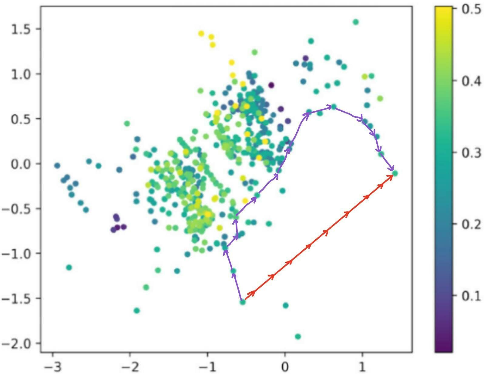

1 Image modified from ChemNav: An interactive visual tool to navigate in the latent space for chemical molecules discovery (www.doi.org/10.1016/j.visinf.2024.10.002).
2 Image from ChemNav: An interactive visual tool to navigate in the latent space for chemical molecules discovery (www.doi.org/10.1016/j.visinf.2024.10.002).
Dead zones in (a subspace of) the latent space. The Euclidean interpolation (red) visits degenerate latent embeddings, while slerp traces a path through the regions where there is valid data.
| Model | Creator | Train size | Representation | Year |
|---|---|---|---|---|
| Molformer-XL | IBM | 1.1 bn | SMILES | 2022 |
| MegaMolBART | NVIDIA | 1.45 bn | SMILES | 2021 |
| ChemBertA | Reverie Labs | 77 mn | SMILES | 2020 |
| Chemformer | AstraZeneca | 100 mn | SMILES | 2021 |
| MolE | Recursion Pharma | 1.2 mn | Graphs | 2022 |
Pre-training methodology: Self-supervised learning like masked language modelling.
Evaluation: MoleculeNet benchmarks (incl. property prediction) & Therapeutic Data Common benchmarks.
Foundation Models
Open questions: But what about their latent spaces? are they contiguous, smooth, regular? how to traverse them efficiently?
Foundation Models
- Chemical foundation models like Chemformer, MolBART do not use stochastic latent variables, but deterministic embeddings.
- You can use embeddings for downstream tasks, but cannot use them for generating new molecules.
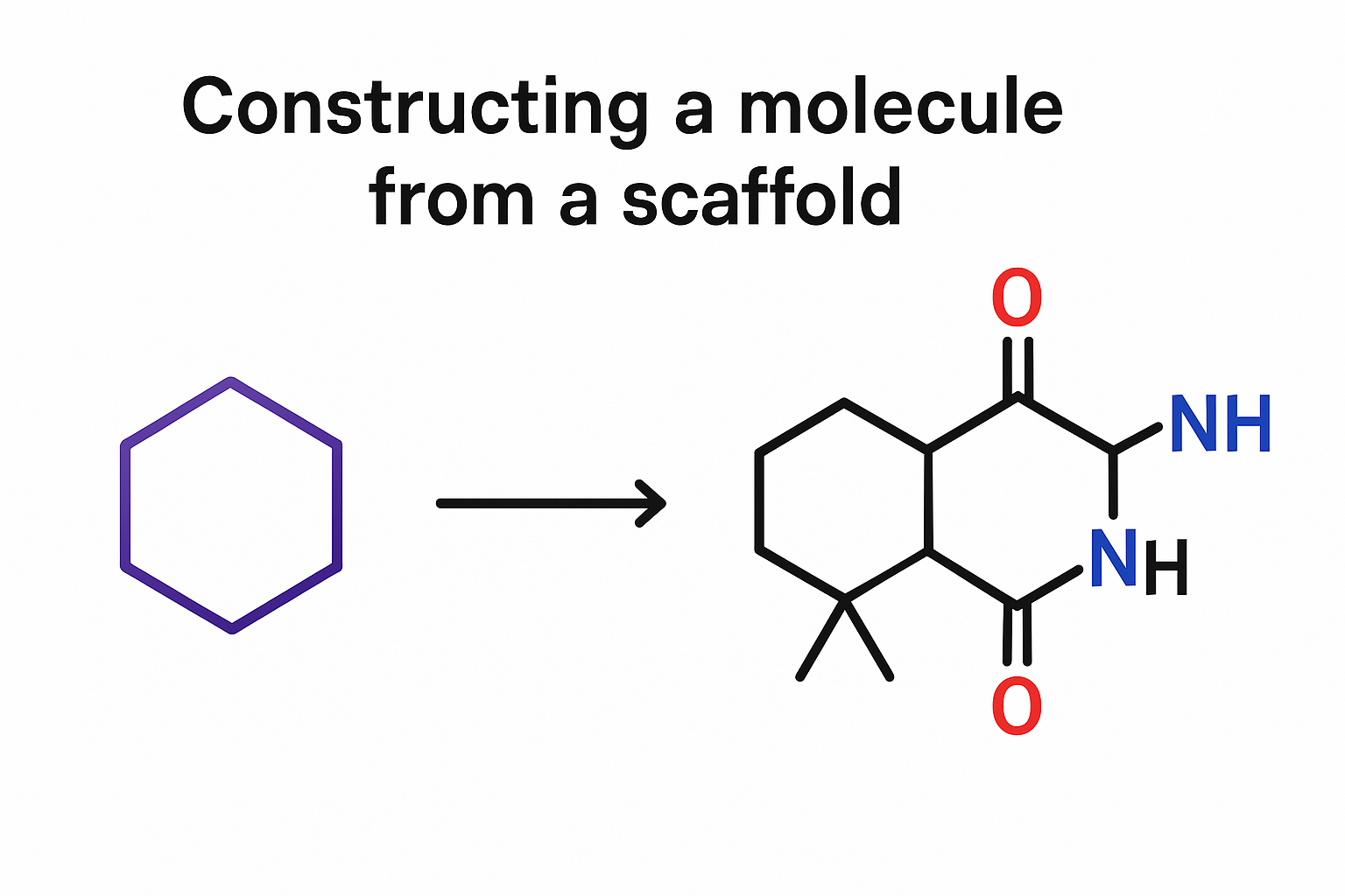
- You have to provide a scaffold or a property and use the decoder to autoregressively construct the sequence from a <START> token.
Key-takeaways
Thank you!
All generative models implicitly learn latent vectors which live on some structured manifold.
-
embedding spaces (e.g. token/patch embeddings),
-
latent spaces (in VAEs, diffusion, etc.),
Their representation topology is extremely important, questions like:
Embeddings of large pre-trained models need to be evaluated and studied through the lens of geometry -- curved latent geometry can reflect robustness vs brittleness and different generalisation capabilities.
-
Do similar inputs lie on connected submanifolds?
-
Are there geometric clusters for tasks, concepts, or modalities?
-
What's the intrinsic dimension of representations across layers?
vidrl@mit.edu
vr308@cam.ac.uk
@VRLalchand
The idea of navigating latent spaces is deeply tied to many frontier problems in biomedical ML.