BDU Multi-output Cancer dose response

Scalable Permutation Invariant Multi-Output Gaussian Processes for Cancer Dose Response

The Schmidt Center, Broad Institute of MIT and Harvard$^{1}$, MIT$^{2}$, University of Oslo$^{3}$

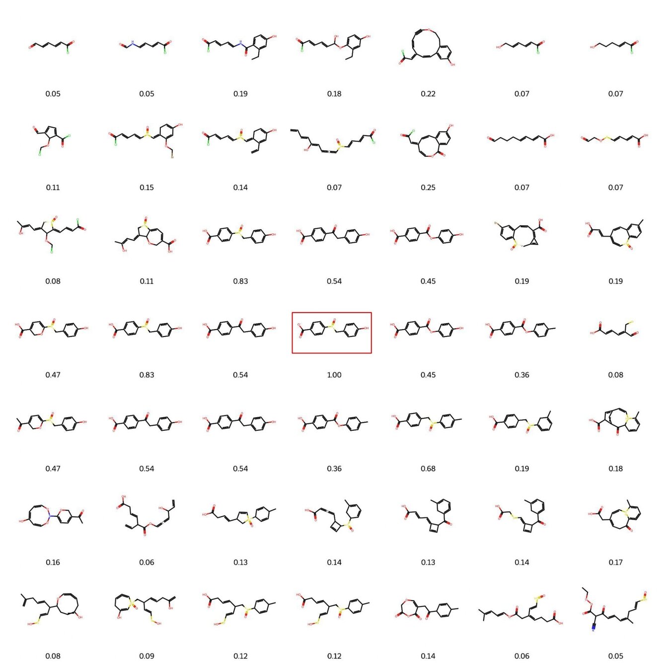
Visualisation of decoded molecules reconstructed from a small neighbourhood around a fixed molecule. The immediate neighbourhood of a known molecule (highlighted in red) yields molecules which share structural similarity – this similarity weakens with increasing Euclidean distance. This underscores the utility of a smooth latent space.

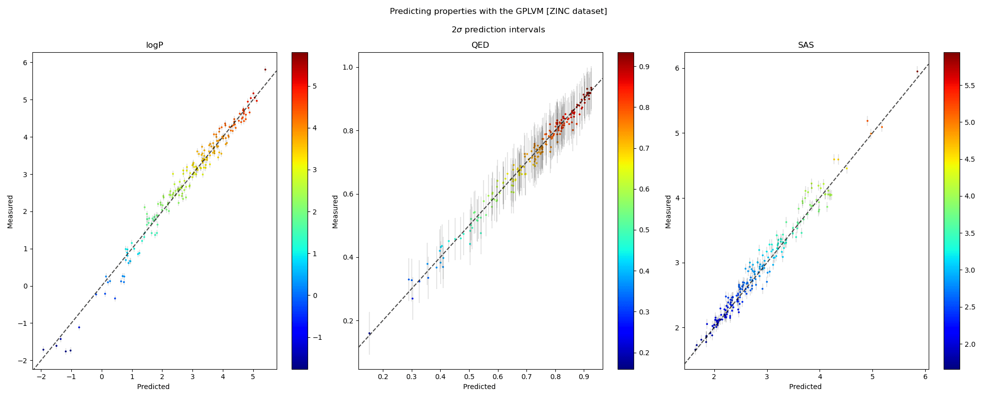
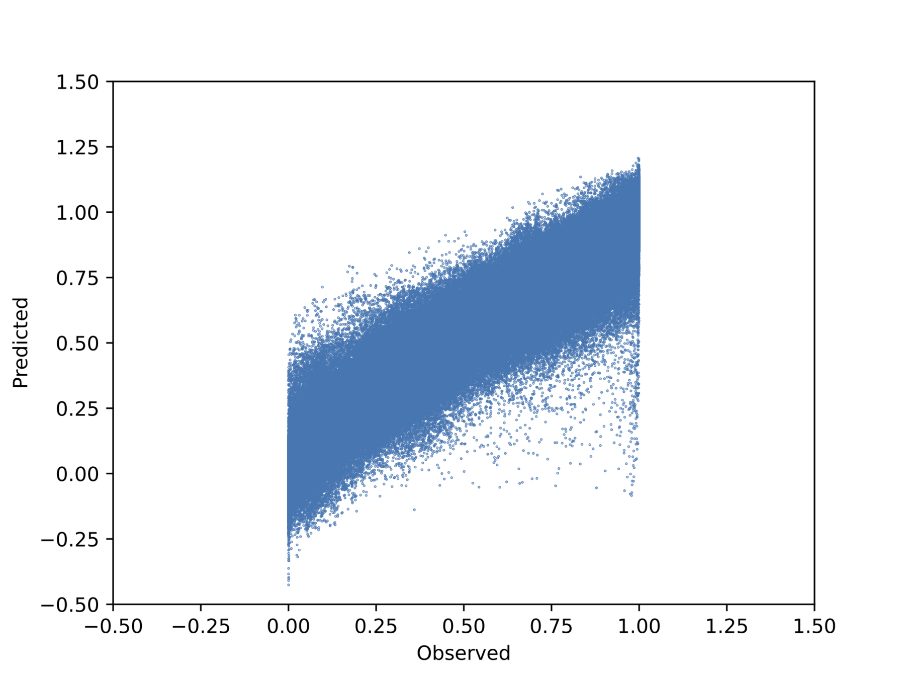
We visualise the predicted and measured property values for each property individually in the plots along a 45° line. The points in the scatter are shaded by the ground truth value of the properties. The grey bars denote 95% confidence intervals approximately corresponding to a $2\sigma$ interval around the mean prediction. We also note the robustness of the prediction intervals as inaccurate predictions are accompanied by wider error bars.

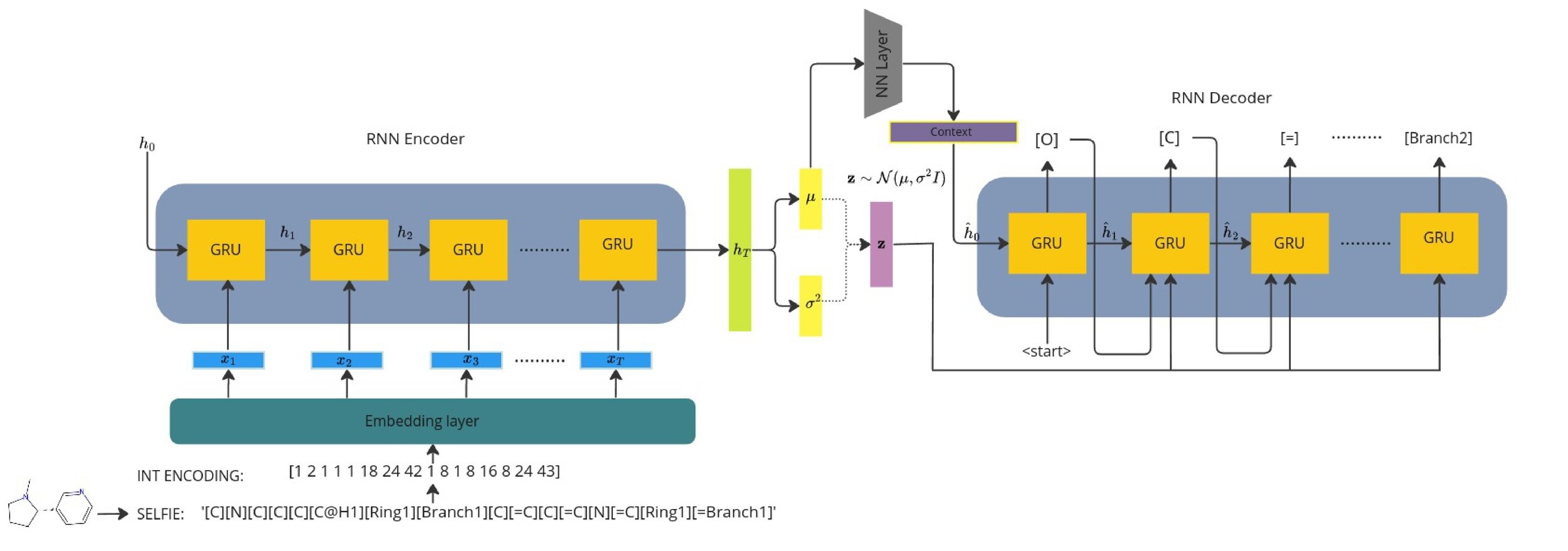
Model Architecture [V-RNN]

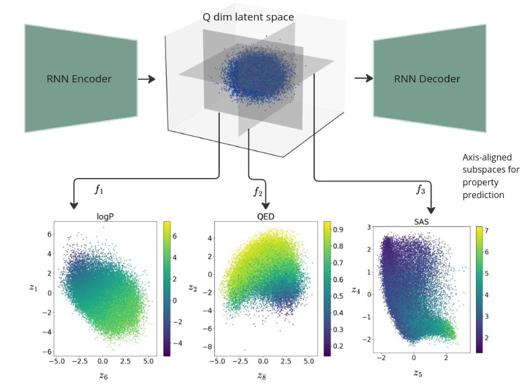
Regularised 2d subspaces per property prediction task. The latent points in each plot are shaded by the ground truth value of the property being modelled by the GP.

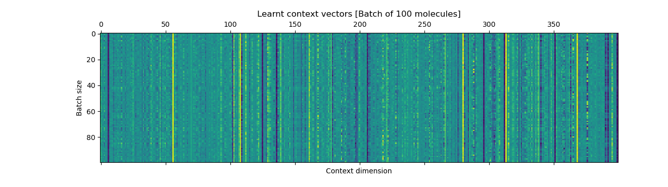
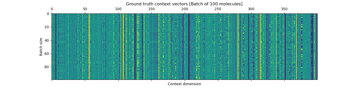
The plots show the ground-truth (right) context vector per data point (row) and the learnt context vector (left) which is learnt during training using an auxilliary fully connected layer which inputs the mean of the latents.

Gaussian Process Decoders for property prediction

1) We learn independent GPs which map from latent space to the property target vector.

3) The GPs are trained jointly with the recurrent VAE to yield smooth subspaces (as a function of target properties) which can be used for gradient based optimisation.

Recurrent VAE with learnt context

2) We use independent SE-ARD kernels inducing automatic pruning of dimensions in latent space.

1) Seq2Seq models typically need a context vector which encodes the context of the whole sequence.

2) This is usually the terminal hidden state of the encoder but we wish to sample and optimise from the continuous latent space.

3) We learn a context vector during training which minimises the error between the terminal encoder hidden state.

Datasets	Structure accuracy [VRNN]	Structure accuracy w. property prediction [VRNN + GPs]
QM9	96.7 (0.11)	94.2 (0.26)
ZINC [250K]	93.8 (0.41)	91.7 (0.55)

Data, Model & Kernel Design

Combination therapies are routinely used in cancer care, as monotherapies are rarely effective.
However, which combinations would benefit cancer patients is largely unknown.
Studies that measure candidate combinations (of drugs) across many cancer cell lines simultaneously can help support combinations research.

Motivation: Drug-synergy modelling

Bliss independence

Multi-output Gaussian process

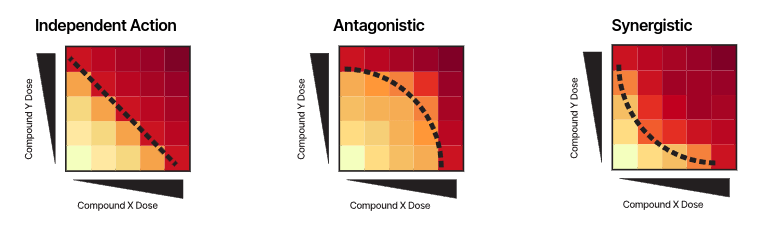
The nature of a drug combination, as synergistic, antagonistic or non-interacting, is usually studied by in-vitro dose–response experiments on cancer cell lines, through e.g. a cell viability assay.

The Bliss model assumes that the two drugs X and Y act independently to achieve their effects.

$E_A$ : The probability of drug $A$ killing a cell.
$E_B$ : The probability of drug $B$ killing a cell.
The probability of neither drug killing a cell is:
$E_A) \cdot (1 - E_B).$
Therefore, the expected viability $V_{XY}$ is, $VABV_{ABV$

$VAB=VA⋅VB,V_{AB} = V_A \cdot V_B,$

$V_{X} = 0.5$ and $V_{Y} =0.6$

$V_{XY} = 0.3$

If $Vobs=0.2V_{\text{obs}} = 0.2$ : Synergy (fewer cells survive than expected).
If $Vobs=0.3V_{\text{obs}} = 0.3$ : Additivity (matches expected survival).
If $Vobs=0.4V_{\text{obs}} = 0.4$ : Antagonism (more cells survive than expected).

(c1, A, B)

(c2, A, B)

(c3, A, B)

(0, 0.11)

(0,0.22)

(0,0.33)

........

(1,1)

$N_{c} \times N_{d} = $ 22,737

$N_{d}$ = 583

$N_{c}$ = 39

$N_{}$ = 100

No. of drug concentrations

No. of cancer cell lines

No. of drug pairs.

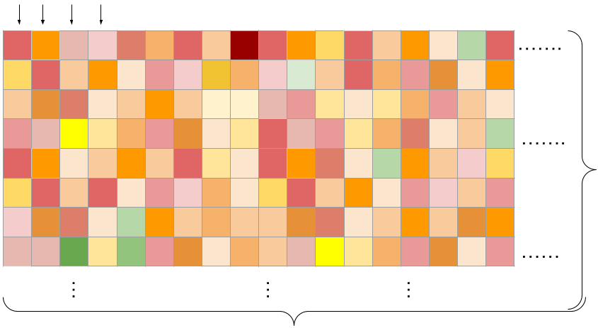
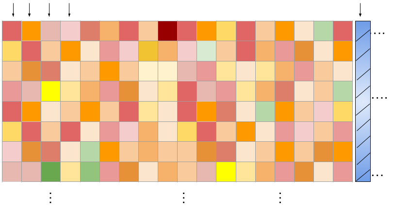
38 drugs were combined in a pairwise manner into 583 distinct combinations that were screened on 39 cancer cell lines yielding a matrix of observations with ~22k columns.

f(\mathbf{x}) = p_{0}(\mathbf{x}) + \Delta(\mathbf{x})

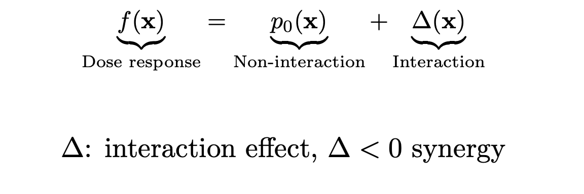
Let $\mathbf{x} = (x_{1}, x_{2})$ denote drug concentrations for an arbitrary pair of drugs, and $h$ denote the single drug dose response, then:

p_{0}(\mathbf{x}) = h_{1}(x_{1})h_{2}(x_{2})

\Delta(\mathbf{x}) = \zeta (g(\mathbf{x}))

g(.) \sim \mathcal{GP}(\mathbf{0}, k(\mathbf{x}, \mathbf{x}^\prime))

Goal: Model the whole matrix as a multi-output Gaussian process with a permutation invariant kernel.

Each output column denotes the dose responses for a triplet denoted by (cell-line (c), drug 1 (A), drug 2 (B)).

We model each output with an underlying GP $ g_{i}$.

Covariance between any two latent functions:

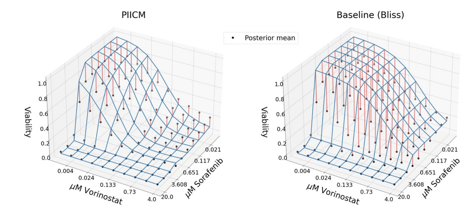
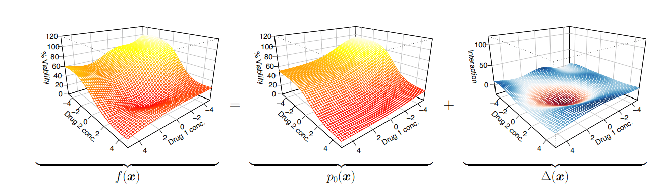
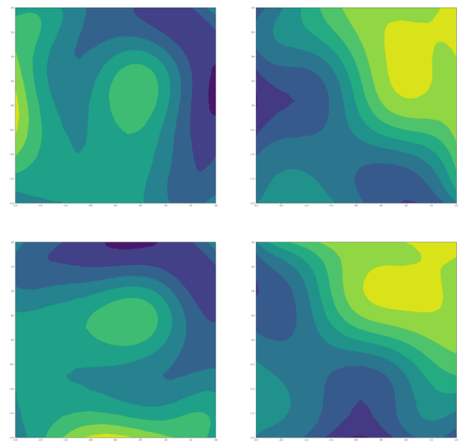
\begin{aligned} \text{Cov}(g_{i}(\mathbf{x}), g_{j}(\mathbf{x}^{\prime})) = \text{Cov}(g_{i}, g_{j})\text{Cov}(\mathbf{x}, \mathbf{x}^{\prime}) = k_{g}(g_{i}, g_{j})k_{x}(\mathbf{x}, \mathbf{x}^{\prime}) \end{aligned}

Predicted dose-response surface

Deviation from actual viability

\begin{aligned} g(c,A,B,{\textbf{x}}) \sim \mathcal{G}\mathcal{P}\left( 0,k _{c}(c,c')\kappa _{d}((A,B),(A',B'))k _{x}({\textbf{x}},{\textbf{x}}')\right) \end{aligned}

Output covariance $k_{g}$ can be further decomposed giving the final multi-ouput GP prior.

\text{vec}(\mathbf{G}) \sim \mathcal{N}(\mathbf{0}, K_{c}\otimes K_{d} \otimes K_{x})

$K_{c}$ is of dimension $ N_{c} \times N_{c}$

$K_{d}$ is of dimension $ N_{d} \times N_{d}$

$K_{x}$ is of dimension $ N \times N$

Cell line covariance: $K_{c} = L_{c}L_{c}^{T} + \text{diag}(\mathbf{v}_{c})$ (free-form low-rank)

Drug pair covariance: $K_{d} = L_{d}L_{d}^{T} + \text{diag}(\mathbf{v}_{d})$ (free-form low-rank)

Drug concentration (input) covariance: $ k(\mathbf{x}, \mathbf{x}') = \sigma_f^2 \exp\left(-\frac{\|\mathbf{x} - \mathbf{x}'\|^2}{2\ell^2}\right) $

g(c,A,B,{\textbf{x}}) \neq g(c,B,A,\tilde{\textbf{x}})

(c, A, B, \mathbf{x}) \rightarrow (c, B, A, \tilde{\mathbf{x}})

We want themapping

\tilde{\mathbf{x}}=(x_2,x_1)

with

to leave the function unchanged

g(c,A,B,(x_{1}, x_{2})) = \tilde{g}(c,A,B,(x_{1}, x_{2})) + \tilde{g}(c,B,A,(x_{2}, x_{1}))

Samples of two permutation invariant functions (reflected across 45$^{\circ}$ line.) modelled by the kernel.

Permutation Invariant formulation

Observed vs. predicted pointwise (unseen outputs)

vidrl@mit.edu, ltronneb@math.uio.no

Vidhi Lalchand$^{1,2}$, Leiv Rønneberg$^{3}$

(no way to distinguish these experiments)

with

Modelling Cancer Drug Response Surfaces with Gaussian Processes

Bliss independence

Multi-output Gaussian process

Theory

Model

The Bliss model of independent action assumes that the two drugs X and Y act independently to achieve their effects.

Observed Viabilities

If $Vobs=0.2V_{\text{obs}} = 0.2$ : Synergy (fewer cells survive than expected).
If $Vobs=0.3V_{\text{obs}} = 0.3$ : Independence (matches expected survival).
If $Vobs=0.4V_{\text{obs}} = 0.4$ : Antagonism (more cells survive than expected).

$V_{X} = 0.5$, $V_{Y} =0.6$

$V_{XY} = 0.3$

https://theprismlab.org/white-papers/multiplexed-cancer-cell-line-combination-screening-using-prism

Let $V_{i}$ denote cancer cell line viability under monotheray $i$

Independent action

Represent dose reponse as a sum of independent + non-linear interaction effects

Vidhi Lalchand, Leiv Ronneberg

Multi-task learning approach

The training data represents (cell line x drug pair) viability measurements across a grid of concentrations. We learn across cell-lines and drugs!

(c1, A, B)

(c2, A, B)

(c3, A, B)

(c*, A*, B*)

Predict at a new (cell-line, drug-pair combination)

$N_{c} \times N_{d} = $ 22,737 (cell-line x drug pair)