How Deep Networks learn Hierarchical and Sparse Data

Based on:
- Failure and success of the spectral bias prediction for Laplace Kernel Ridge Regression: the case of low-dimensional data [ICML 22]
- How deep convolutional neural network lose spatial information with training, [ICLR23 Workshop], [Machine Learning: Science and Technology 2023]
- How deep convolutional networks learn compositional data: the Random Hierarchy Model, [PRX]
- How Deep Networks Learn Hierarchical and Sparse Data, [ICML 24]
Umberto Maria Tomasini
The puzzling success of Machine Learning
- Machine learning is incredibly successful across tasks
- Curse of dimensionality when learning in high dimensions
vs.
- Data must be structured
- Machine Learning should capture such structure of data
\(P\): training set size
\(d\) data-space dimension
Which aspects of real data make them learnable?
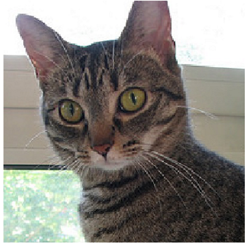
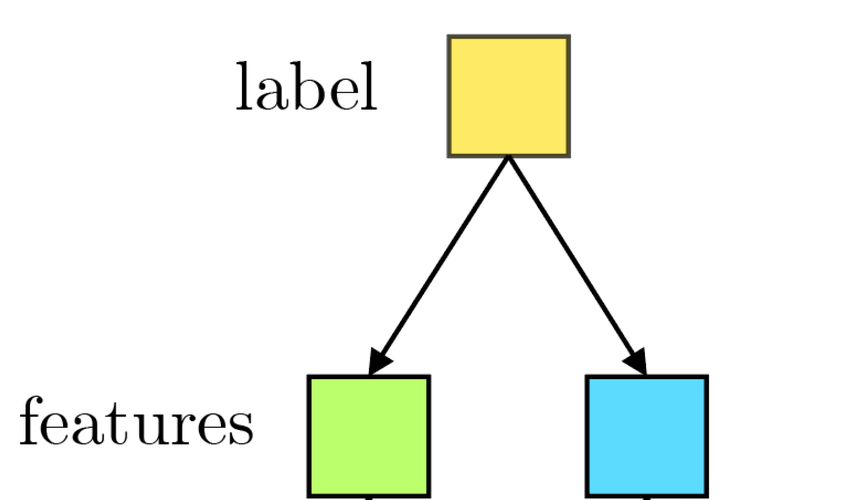
Cat
The cat is _____ \(\Rightarrow\) grey
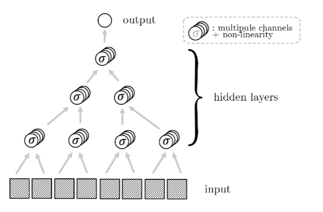
- Hierarchical structure: data are made by features organized hierarchically. High-level features are made of low-level features.
A property of data that may be leveraged by networks
sofa
- There are equivalent low-level representations for the same high-level feature, called synonyms
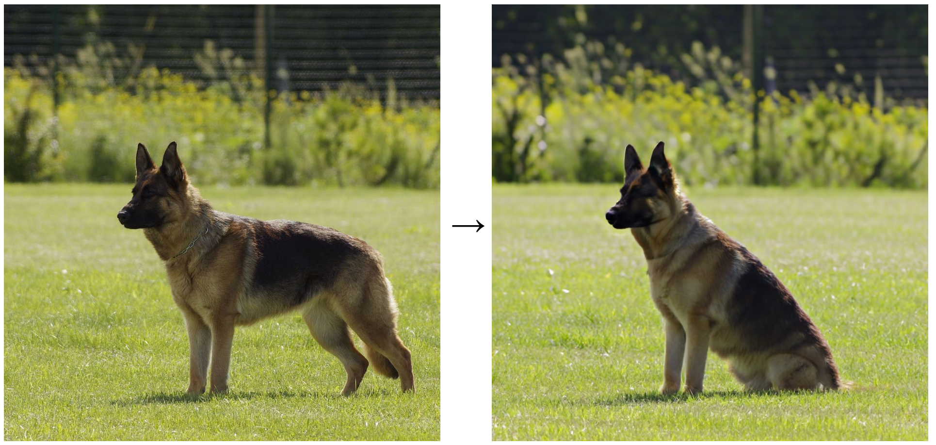
Image by [Kawar, Zada et al. 2023]
The cat sat on the sofa
The cat sat on the couch
Our approach:
- Present a model of data that captures the hierarchical structure.
- Deep networks beat the curse of dimensionality learning the model.
- The network representations have learnt the structure of the task.
Is hierarchy learnt by networks?
Hierarchical Generative Models
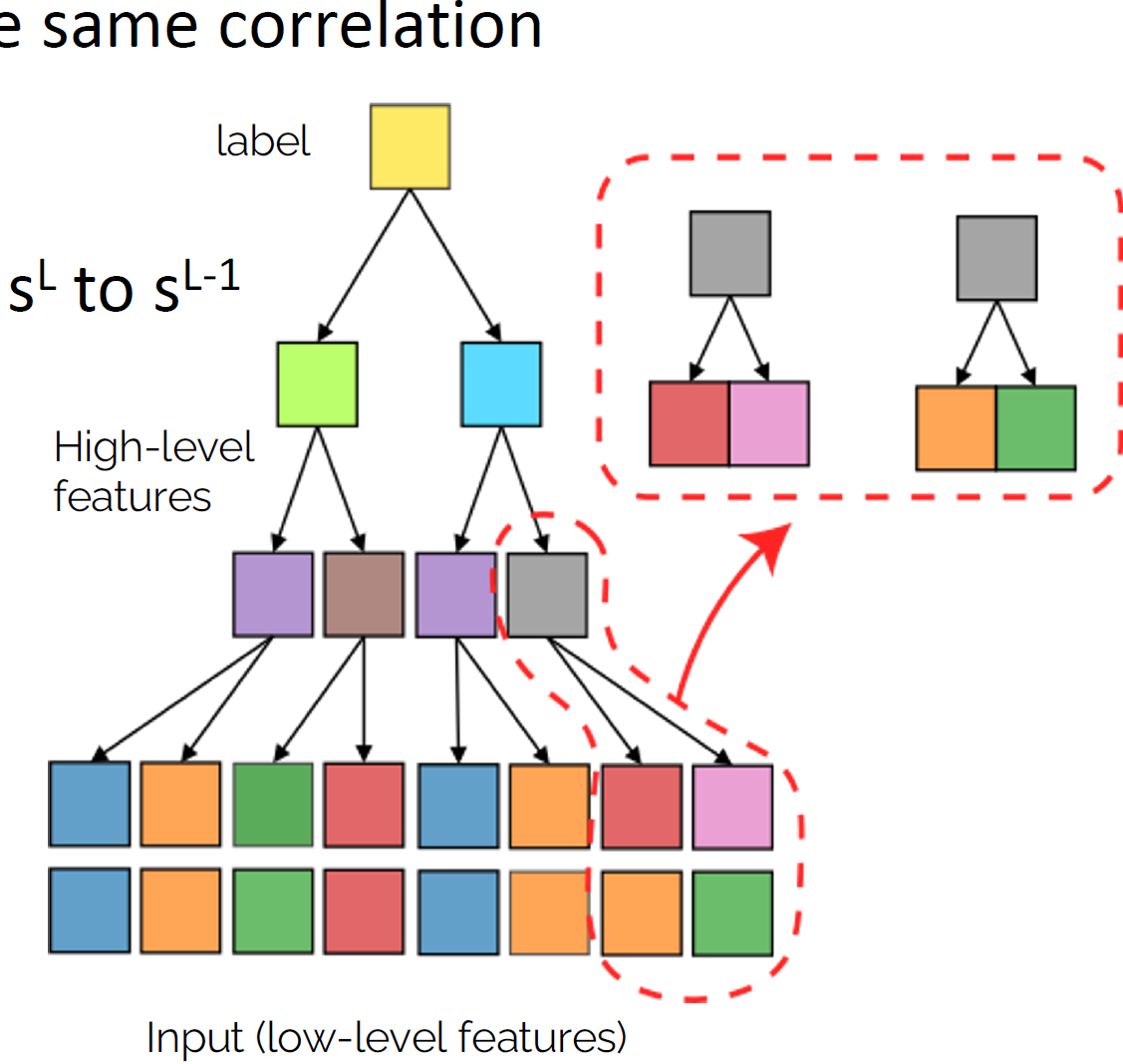
- Number of colors: \(v=\{\text{Blue}, \text{Orange}...\}\)
- Number of classes: \(n_c\)
- Patch size: \(s\)
Synonyms
\(m=2\)
\(L\): depth
sofa
\(\frac{1}{2}\)
\(\frac{1}{2}\)
\(\frac{1}{2}\)
\(\frac{1}{2}\)
\(\frac{1}{2}\)
\(\frac{1}{2}\)
\(\frac{1}{2}\)
\(\frac{1}{2}\)
Rules Level 1
Rules Level 2
\(\Rightarrow\)
Sampled examples
Hierarchical Generative Models
Synonyms
\(L\): depth
(here \(L=2\))
\(s\): patch dimension
(input dimension \(s^L\))
Label 1
Label 2
\(m=2\)
Number classes
\(n_c =2\)
'How deep convolutional networks learn hierarchical tasks: the Random Hierarchy Model'
Number of features (colors) \(v=2\)
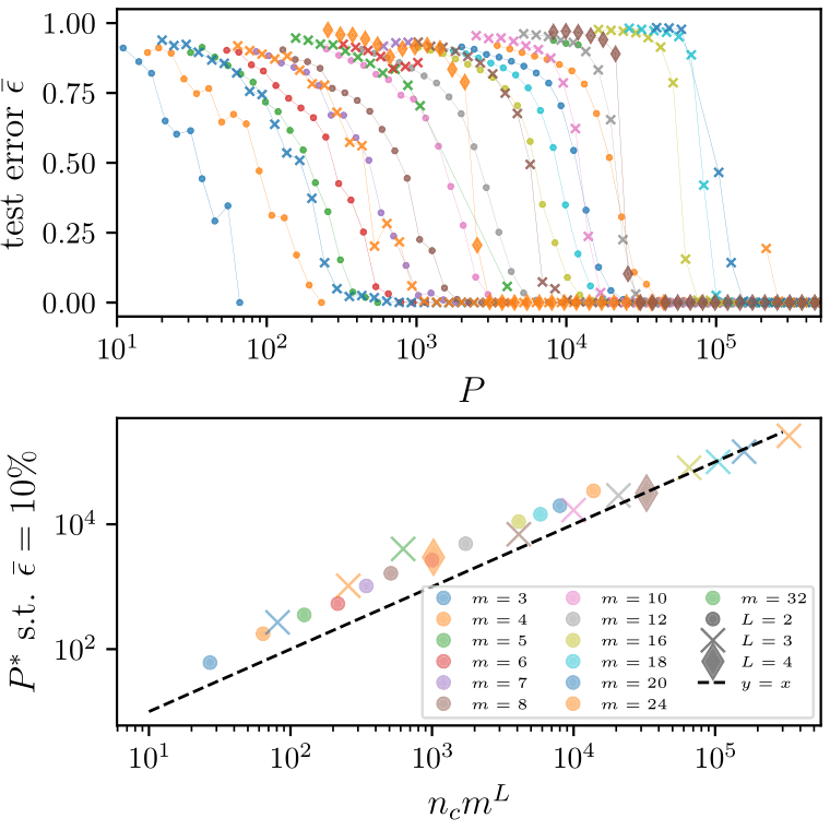
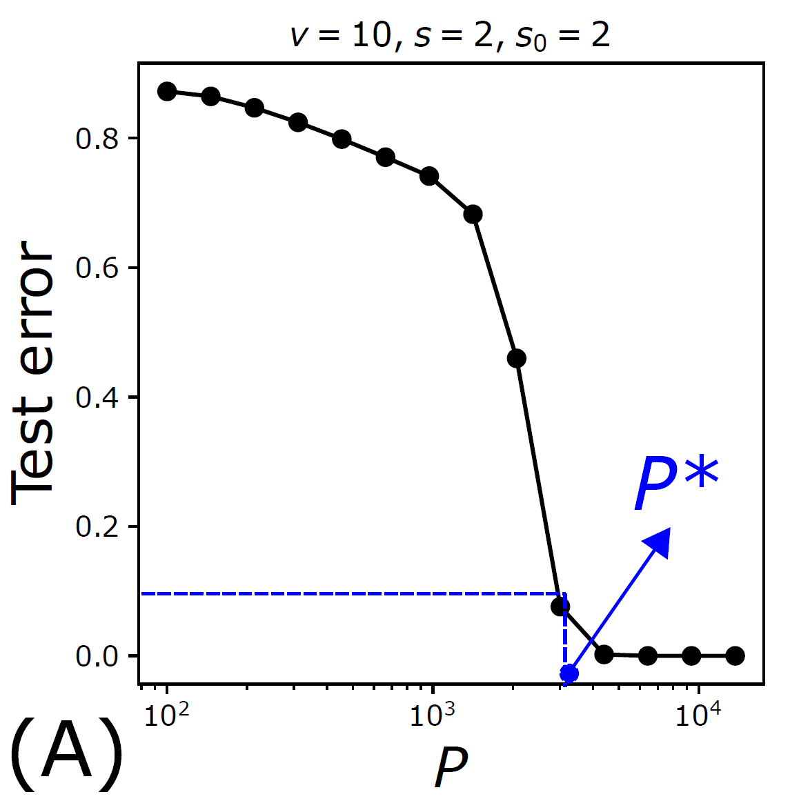
Deep networks beat the curse of dimensionality
\(P^*\)
\(P^*\sim n_c m^L\)
- Polynomial in the input dimension \(s^L\)
- Beating the curse
- Shallow network \(\rightarrow\) cursed by dimensionality
- Depth is key to beat the curse, learning deep data structure
How deep networks learn the hierarchy?
- Intuition: learn the group of synonyms of low-level patches, encoding for the same high-level feature;
- Leveraging on the fact that the synonyms have equal correlation with the label;
- Going one level up in the hierarchy;
- Iterate \(L\) times up to the label.
Learning the task happens when synonyms are learnt.
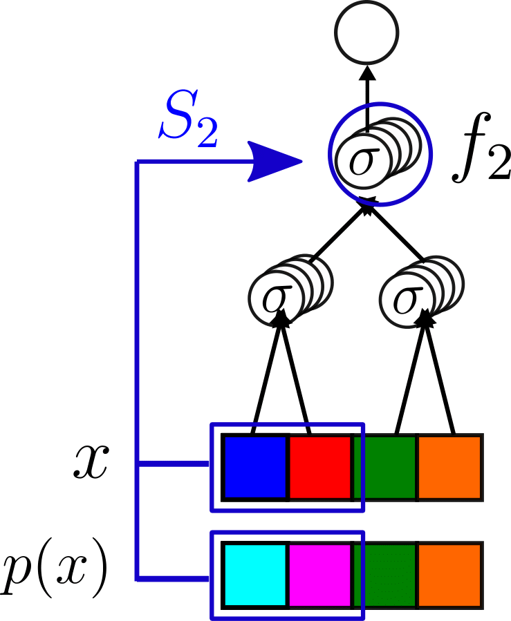
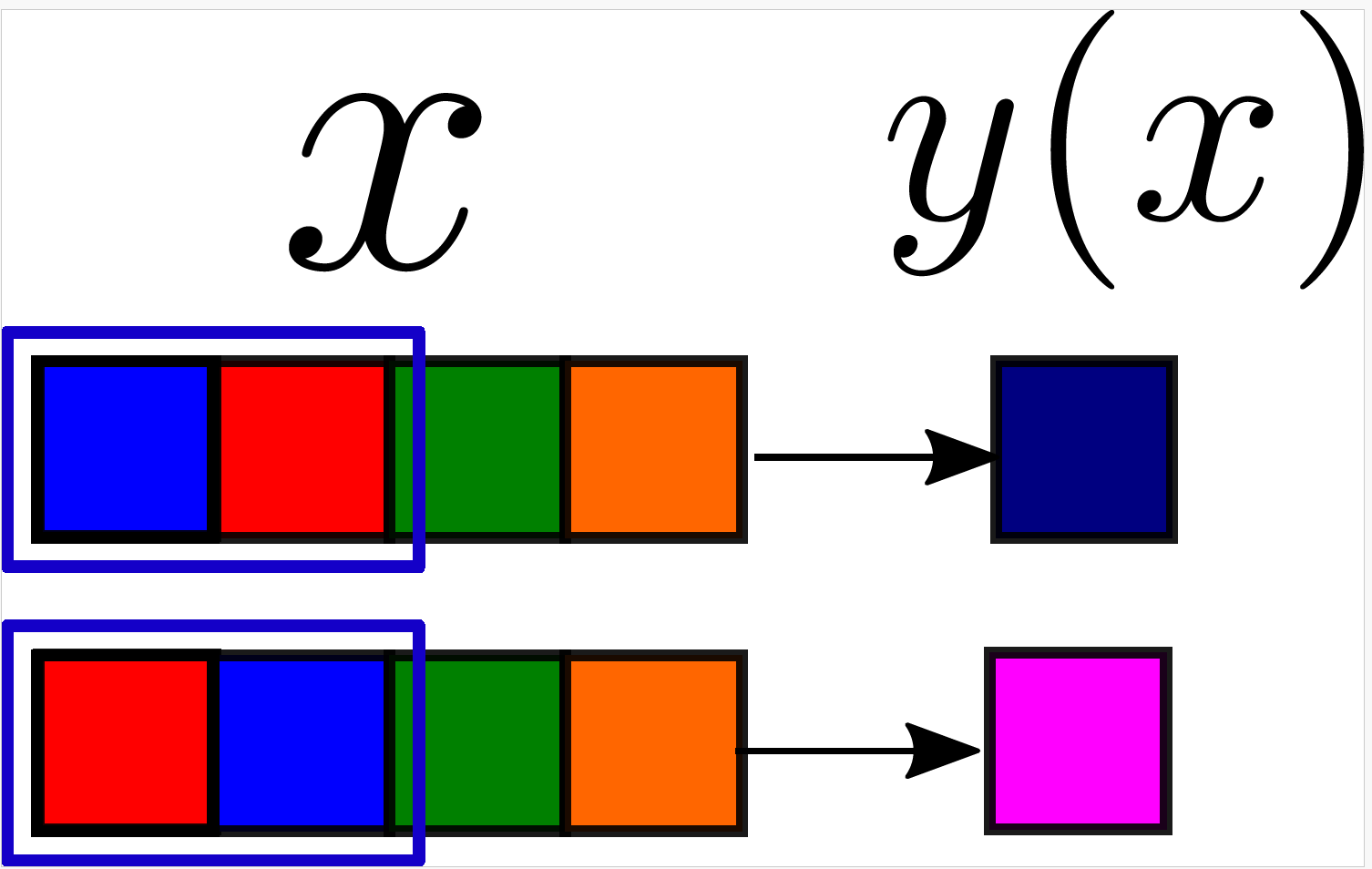
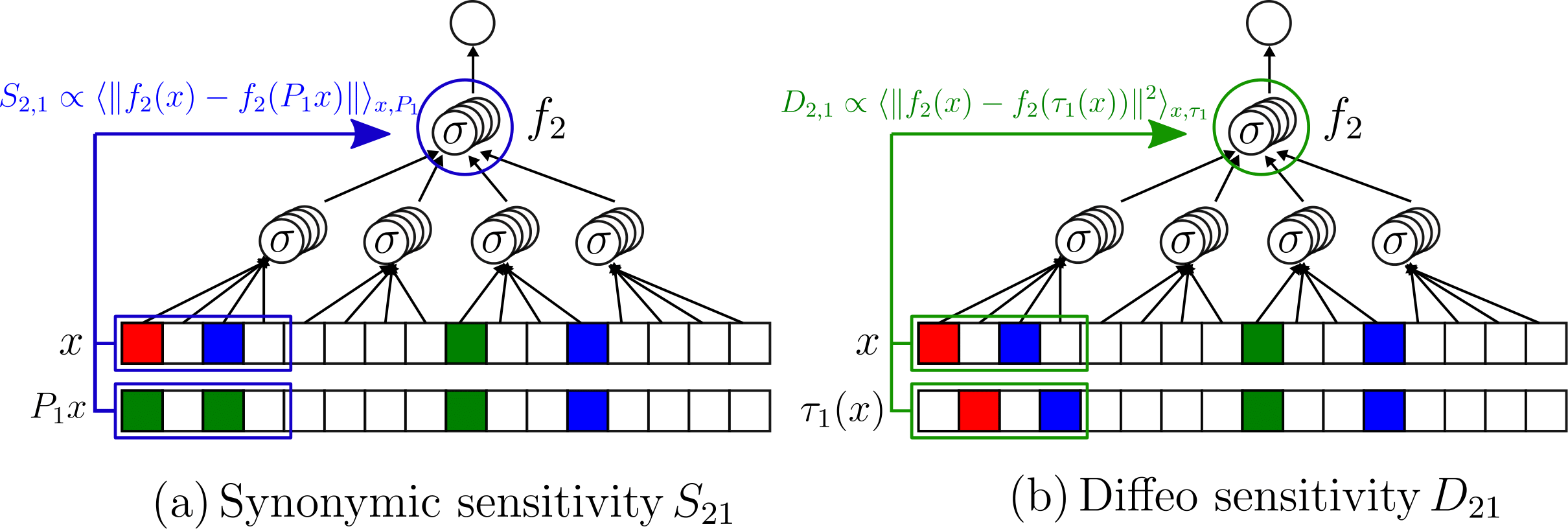
- We take a trained CNN
- We apply a synonyms exchange \(p\) on a input datum \(x\);
- We check whether the second network layer \(f_2\) is sensitive to it:
\(S_2\propto \langle||f_2(x)-f_2(p(x))||^2\rangle_{x,p}\)
How to measure if networks learn the hierarchy
Also synonyms learnt at \(P^*\)
Takeaways
- Deep networks learn hierarchical tasks
- They do so by developing internal representations invariant to synonyms exchange
Limitations
- Not fully capturing the structure of images
- Images are sparse
- In classification, the exact position of the features does not matter
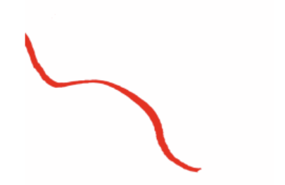
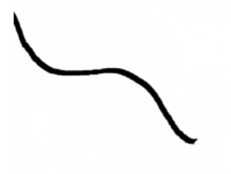
- \(\rightarrow\) invariance to smooth transformations like diffeomorphisms
- Deep networks learn to become insensitive to diffeomorphisms with training. [Petrini21]
- [Tomasini2023]: deep networks achieve so by learning a series of pooling operations.
- Learning diffeomorphisms correlates with performance!
Invariance to Diffeomorphisms is central in image classification
Questions
- Why is there such a correlation?
- Are networks learning also the hierarchical structure? Does it correlate with performance?
- If yes, with how many training points?
- To answer these questions, we propose an extension of our hierarchical model
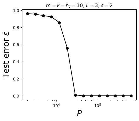
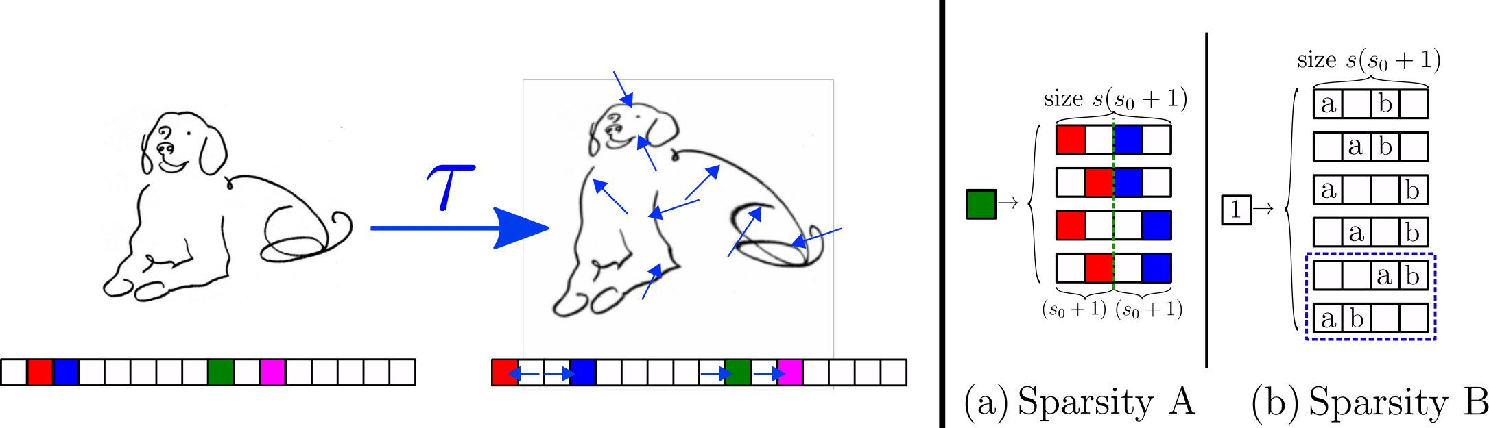
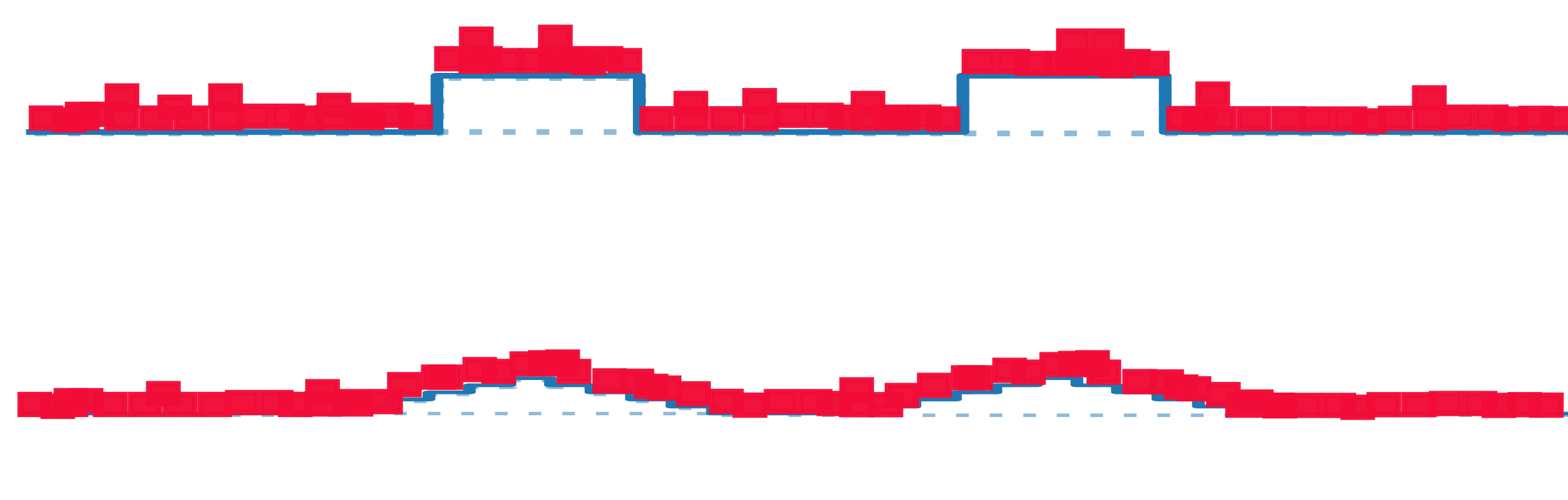
Sparse Hierarchical Random Model
- Keeping the hierarchical structure
- Adding meaningless \(s_0\) pixels '0' around each feature, at each hierarchy level.
- The meaningless pixels '0' are in random positions.
\(\textcolor{blue}{s_0=2}\)
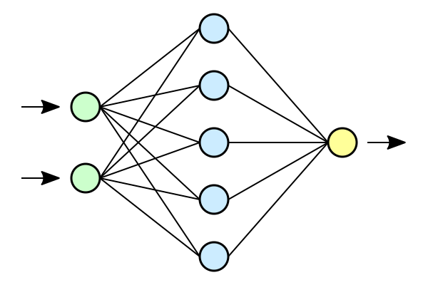
Which net do we use?
We consider a different version of a Convolutional Neural Network (CNN) without weight sharing
Standard CNN:
- local
- weight sharing
Locally Connected Network (LCN):
- local
weight sharing
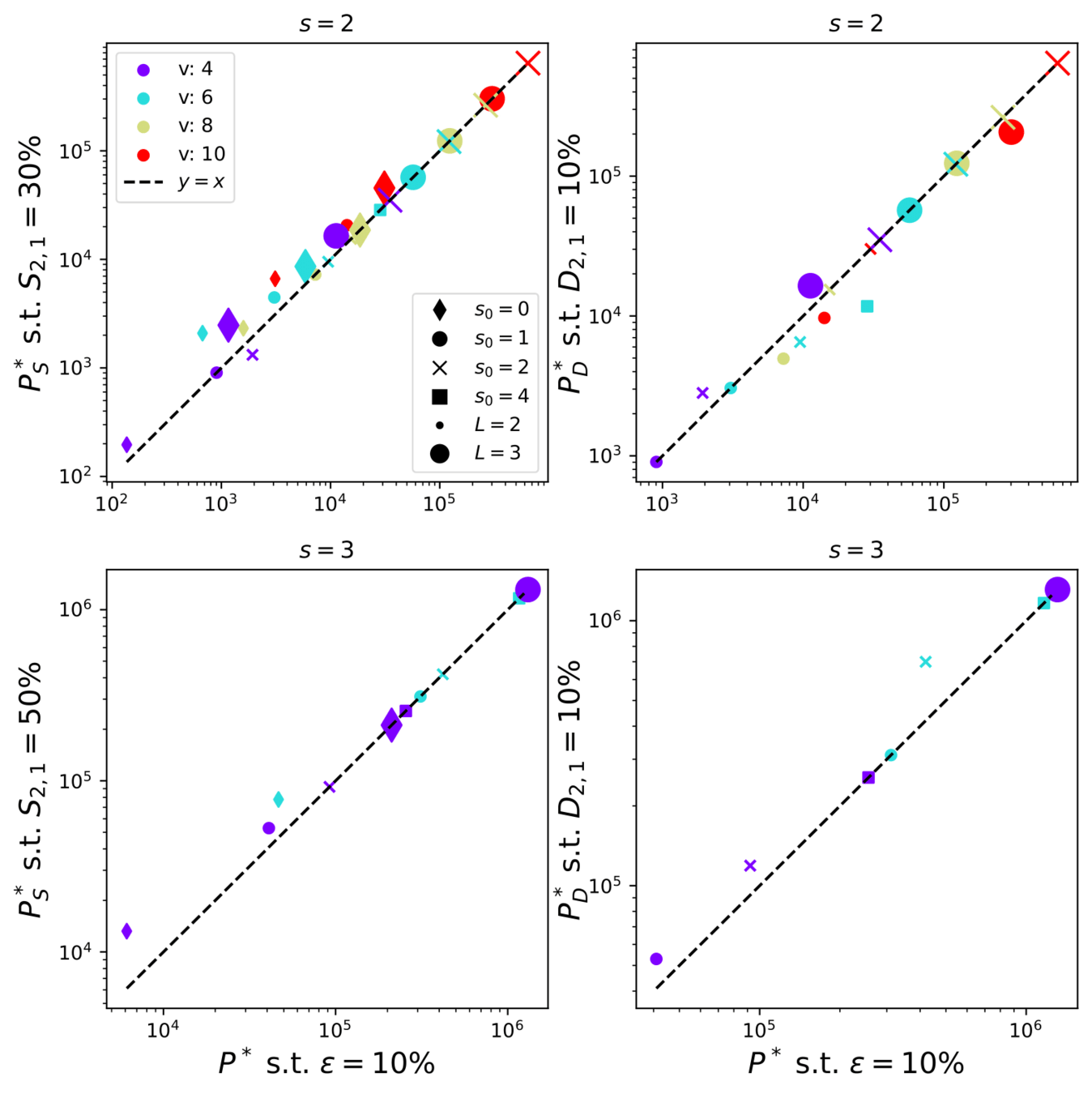
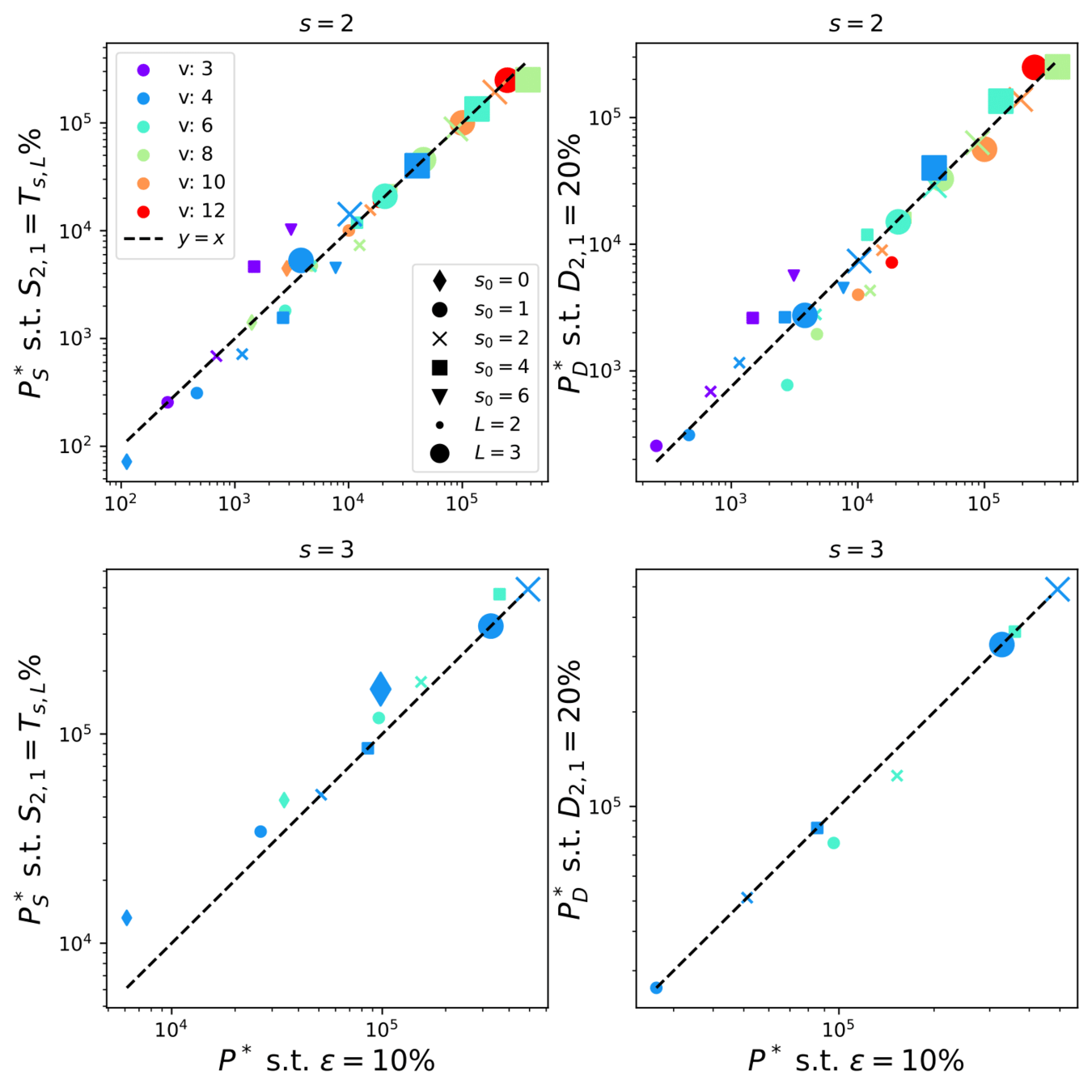
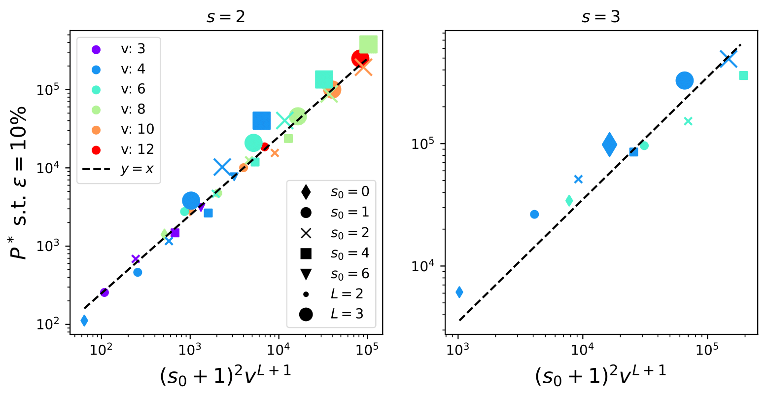
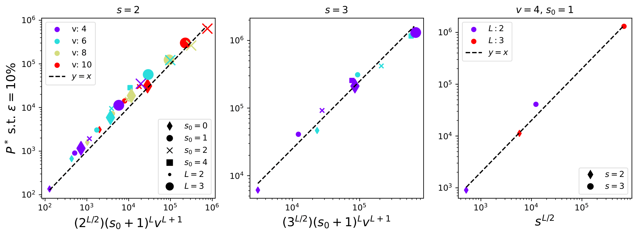
How many training points to learn the task?
- Polynomial in the input dimension \([s(s_0+1)]^L\)
- Beating the curse
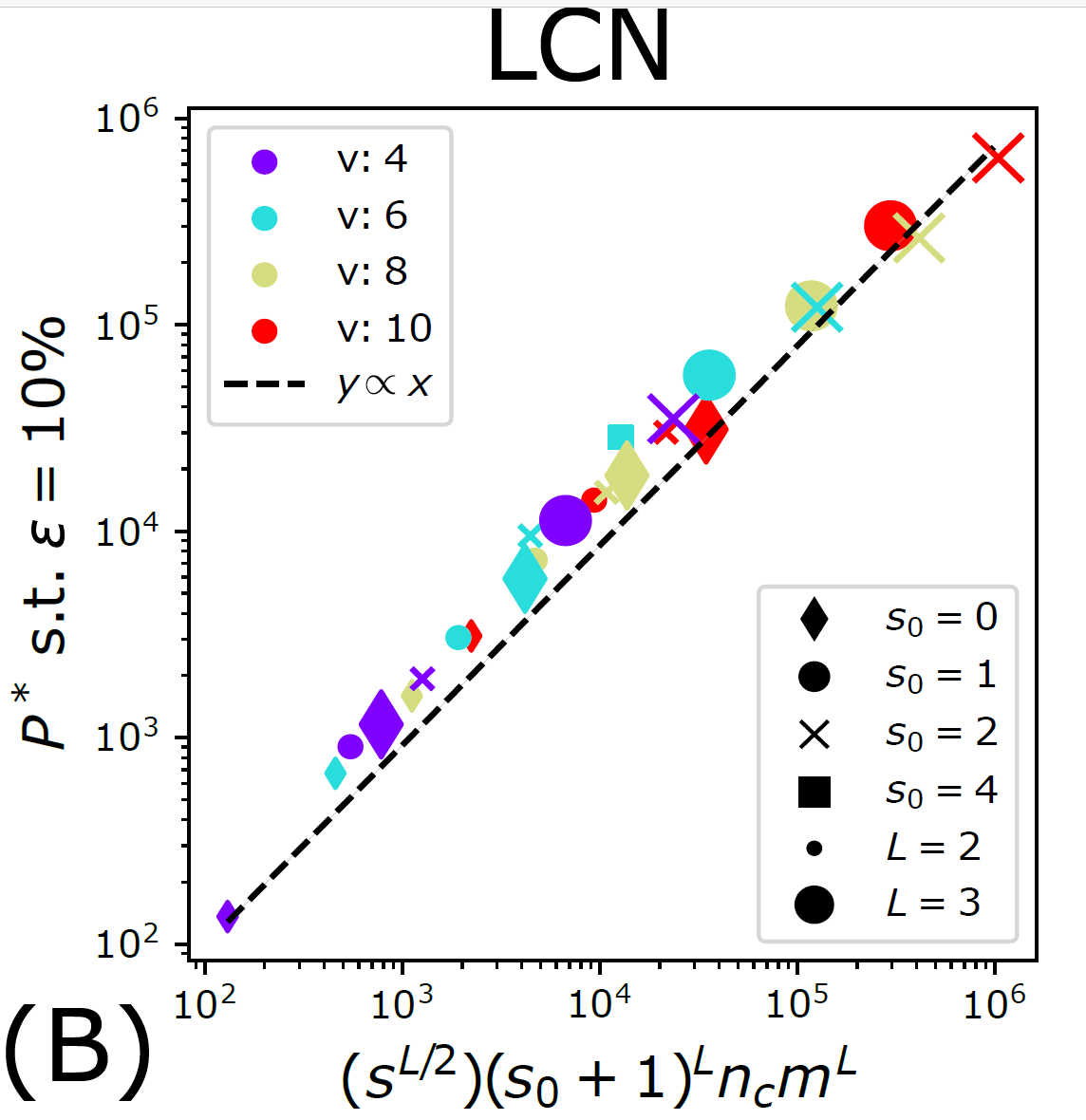
\(P^*\sim \textcolor{blue}{(s_0+1)^L}n_c m^L\)
How many training points?
- Without sparsity (\(s_0=0\)): \(P^*_0\sim n_c m^L\)
- With sparsity, for most of the data, a local weight does not see anything.
\(\Rightarrow\)To recover the synonyms and then solve the task,
it is then necessary to see many more data:
\(P^*_{\text{LCN}}\sim (s_0+1)^L P^*_0\)
\(s_0=1\)
Probability to see a signal in a given location:
\(p=\frac{1}{(s_0+1)^L}\)
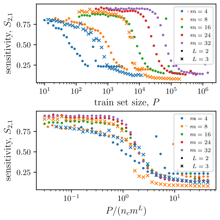
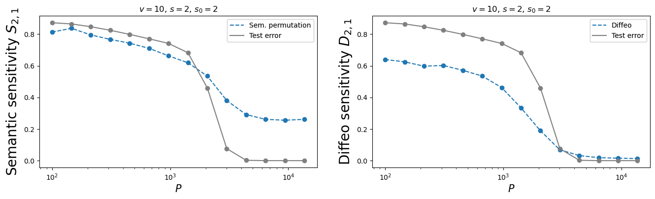
- We take a 2-layer LCN, trained on the sparse hierarchical dataset (with \(v=m\) and \(L=2\)) with \(P\) training points;
- We apply either synonyms exchange or diffeo on the input data;
- We check whether the second net layer is sensitive to these transformations.
Testing synonymic and diffeo sensitivity
2
Do deep networks learn the data structure?
Diffeomorphisms
learnt with the task
Synonyms learnt with the task
The hidden representations become insensitive to the invariances of the task
Why are diffeo and synonyms learnt together?
Since a network reconstructs the hierarchical task by leveraging patch-label correlations, the synonyms and their spatial rearrangements are grouped together, yielding invariance to diffeo.
\(x_1\)
\(x_2\)
\(x_3\)
\(x_4\)
Why the best networks are the most insensitive to diffeomorphisms
A hierarchical representation, crucial for achieving good performance, is learnt precisely at the same number of training points at which insensitivity to diffeomorphisms is achieved.
Takeaways
- Deep networks beat the curse of dimensionality on sparse hierarchical tasks.
- The hidden representations become insensitive to the invariances of the task: synonyms exchange and spatial smooth transformations.
Look whether also deep networks trained on real data learn invariant representations together with the task.
Future directions
Image by [Kawar, Zada et al. 2023]
Thank you!
[Sclocchi, Favero 24]
BACKUP SLIDES
Do deep networks learn the data structure?
Diffeomorphisms
learnt with the task
Synonyms learnt with the task
How to learn the Hierarchy?
- Intuition: learn the group of synonyms of low-level patches, encoding for the same high-level feature;
- Leveraging on the fact that the synonyms have equal correlation with the label;
- Going one level up in the hierarchy;
- Iterate \(L\) times up to the label.
Learning the task happens when synonyms are learnt.
Number of training points needed: \(P^*\sim (s_0+1)^L n_c m^L\)
Why are diffeo and synonyms learnt together?
If a network reconstructs the hierarchical task by leveraging local feature-label correlations, then it extends this capability at each equivalent location, yielding invariance to diffeo.
\(x_1\)
\(x_2\)
The learning algorithm
- Regression of a target function \(f^*\) from \(P\) examples \(\{x_i,f^*(x_i)\}_{i=1,...,P}\).
- Interest in kernels renewed by lazy neural networks
Train loss:
\(K(x,y)=e^{-\frac{|x-y|}{\sigma}}\)
E.g. Laplacian Kernel
- Kernel Ridge Regression (KRR):
Fixed Features
Failure and success of Spectral Bias prediction..., [ICML22]
- Key object: generalization error \(\varepsilon_t\)
- Typically \(\varepsilon_t\sim P^{-\beta}\), \(P\) number of training data
Predicting generalization of KRR
[Canatar et al., Nature (2021)]
General framework for KRR
- Predicts that KRR has a spectral bias in its learning:
\(\rightarrow\) KRR learns the first \(P\) eigenmodes of \(K\)
\(\rightarrow\) \(f_P\) is self-averaging with respect to sampling
- Obtained by replica theory
- Works well on some real data for \(\lambda>0\)
\(\rightarrow\) what is the validity limit?
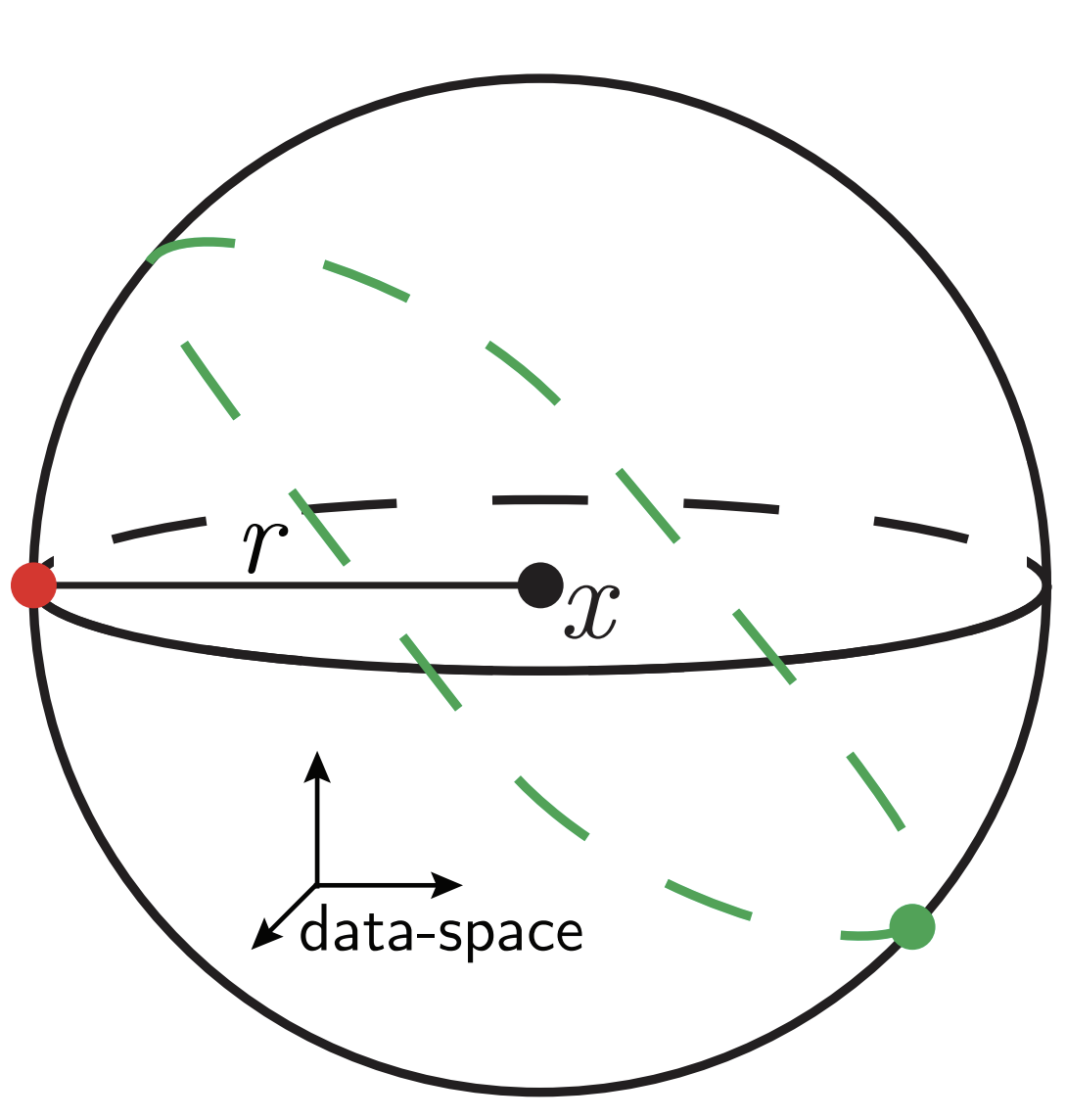
Our toy model
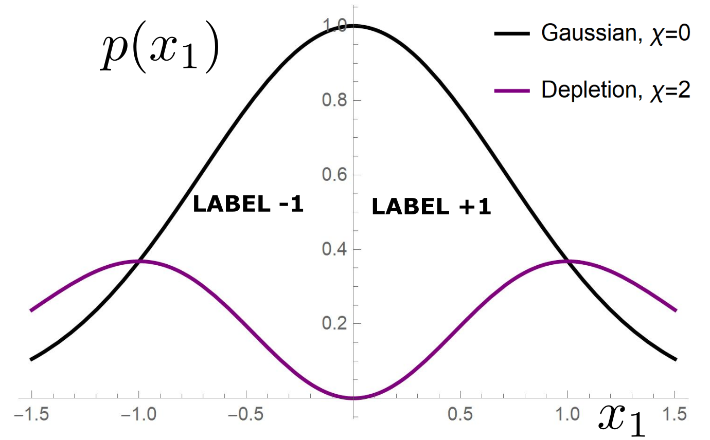
Depletion of points around the interface
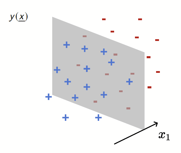
Data: \(x\in\mathbb{R}^d\)
Label: \(f^*(x_1,x_{\bot})=\text{sign}[x_1]\)
Motivation:
evidence for gaps between clusters in datasets like MNIST
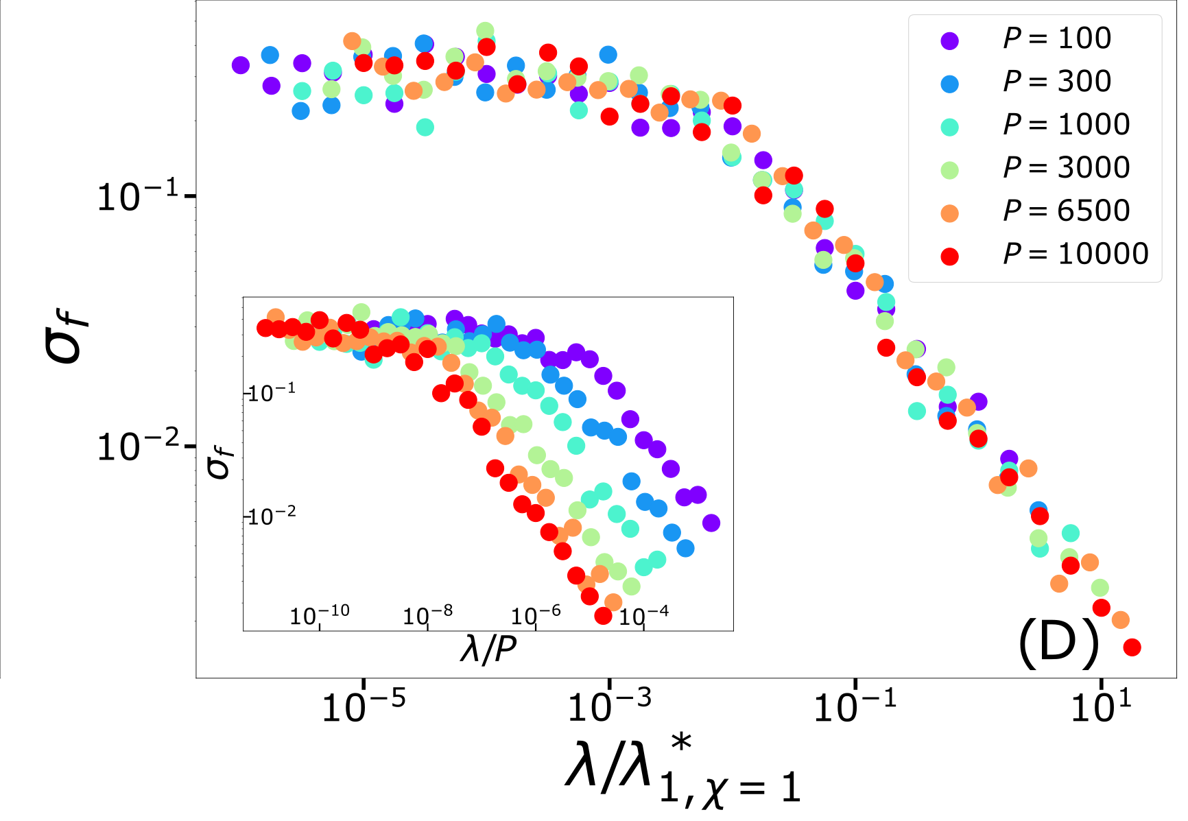
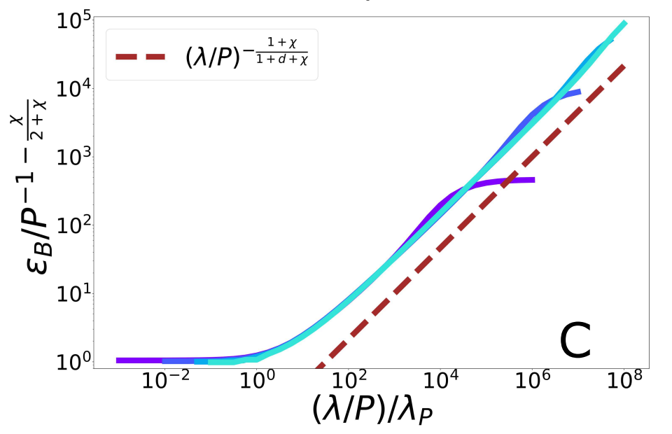
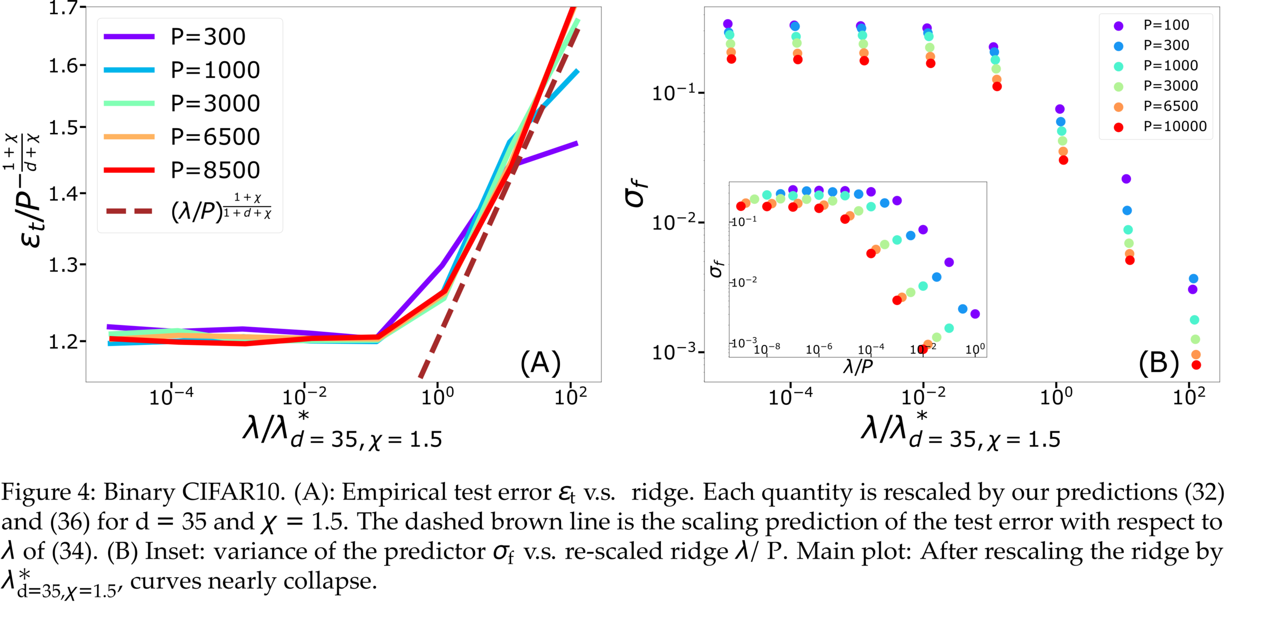
Predictor in the toy model
(1) Spectral bias predicts a self-averaging predictor controlled by a characteristic length \( \ell(\lambda,P) \propto \lambda/P \)
For fixed regularizer \(\lambda/P\):
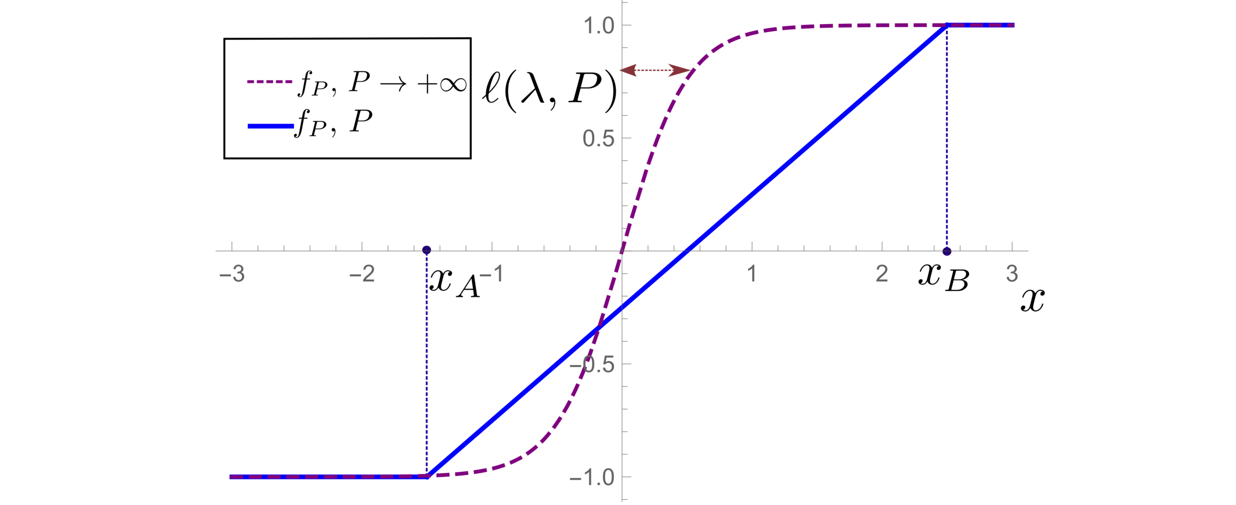
(2) When the number of sampling points \(P\) is not enough to probe \( \ell(\lambda,P) \):
- \(f_P\) is controlled by the statistics of the extremal points \(x_{\{A,B\}}\)
- spectral bias breaks down.
\(d=1\)
Different predictions for
\(\lambda\rightarrow0^+\)
- For \(\chi=0\): equal
- For \(\chi>0\): equal for \(d\rightarrow\infty\)
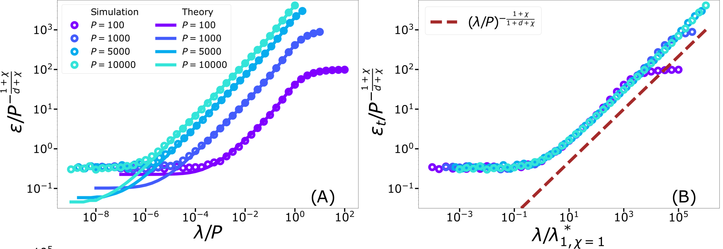
Crossover at:
\(\lambda\)
Spectral bias failure
Spectral bias success
Takeaways and Future directions
For which kind of data spectral bias fails?
Depletion of points close to decision boundary
Still missing a comprehensive theory for
KRR test error for vanishing regularization
- That was our work on the performance of Kernel Methods
- Now: what happens for deep networks learning structured data?
Test error: 2 regimes
For fixed regularizer \(\lambda/P\):
\(\rightarrow\) Predictor controlled by extreme value statistics of \(x_B\)
\(\rightarrow\) Not self-averaging: no replica theory
(2) For small \(P\): predictor controlled by extremal sampled points:
\(x_B\sim P^{-\frac{1}{\chi+d}}\)
The self-averageness crossover
\(\rightarrow\) Comparing the two characteristic lengths \(\ell(\lambda,P)\) and \(x_B\):
Different predictions for
\(\lambda\rightarrow0^+\)
- For \(\chi=0\): equal
- For \(\chi>0\): equal for \(d\rightarrow\infty\)
- Replica predictions works even for small \(d\), for large ridge.
- For small ridge: spectral bias prediction, if \(\chi>0\) correct just for \(d\rightarrow\infty\).
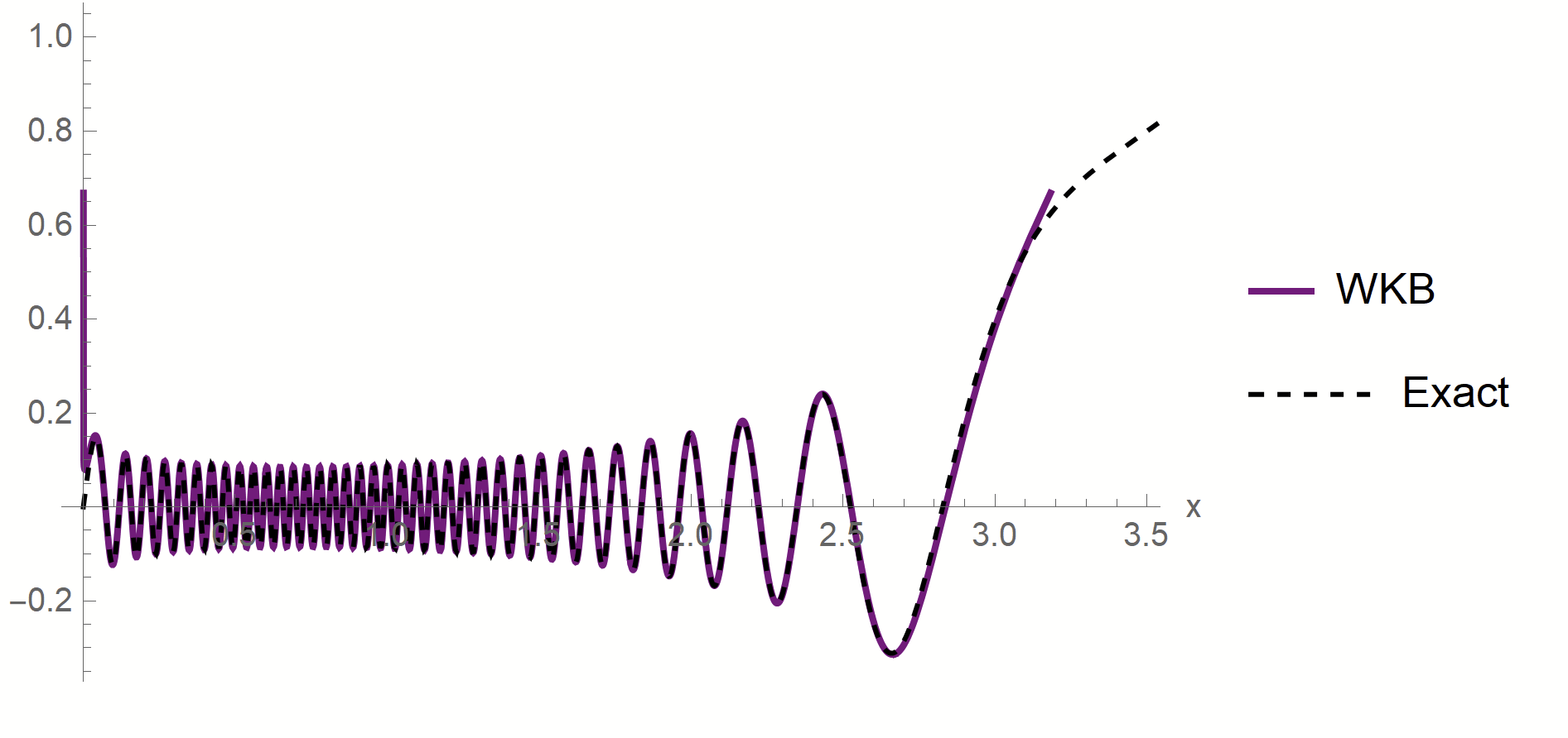
- To test spectral bias, we solved eigendecomposition of Laplacian kernel for non-uniform data, using quantum mechanics techniques (WKB).
- Spectral bias prediction based on Gaussian approximation: here we are out of Gaussian universality class.
Technical remarks:
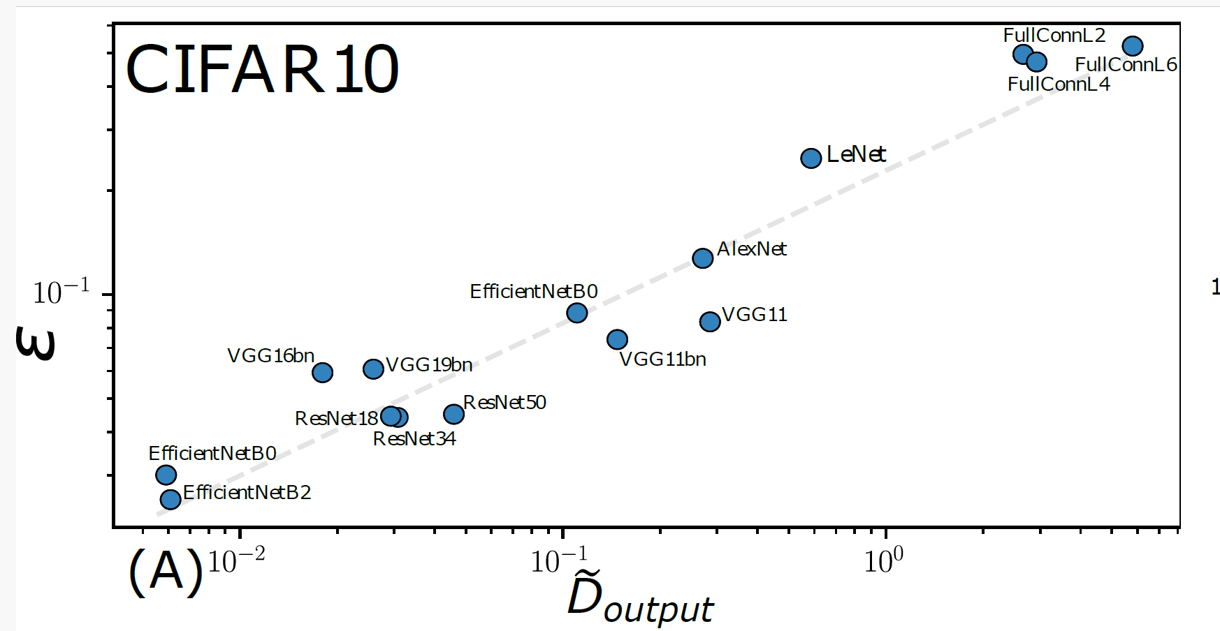
Scaling Spectral Bias prediction
Fitting CIFAR10
Proof:
- WKB approximation of \(\phi_\rho\) in [\(x_1^*,\,x_2^*\)]:
\(\phi_\rho(x)\sim \frac{1}{p(x)^{1/4}}\left[\alpha\sin\left(\frac{1}{\sqrt{\lambda_\rho}}\int^{x}p^{1/2}(z)dx\right)+\beta \cos\left(\frac{1}{\sqrt{\lambda_\rho}}\int^{x}p^{1/2}(z)dx\right)\right]\)
- MAF approximation outside [\(x_1^*,\,x_2^*\)]
\(x_1*\sim \lambda_\rho^{\frac{1}{\chi+2}}\)
\(x_2*\sim (-\log\lambda_\rho)^{1/2}\)
- WKB contribution to \(c_\rho\) is dominant in \(\lambda_\rho\)
- Main source WKB contribution:
first oscillations
Formal proof:
- Take training points \(x_1<...<x_P\)
- Find the predictor in \([x_i,x_{i+1}]\)
- Estimate contribute \(\varepsilon_i\) to \(\varepsilon_t\)
- Sum all the \(\varepsilon_i\)
Characteristic scale of predictor \(f_P\), \(d=1\)
Minimizing the train loss for \(P \rightarrow \infty\):
\(\rightarrow\) A non-homogeneous Schroedinger-like differential equation
\(\rightarrow\) Its solution yields:
Characteristic scale of predictor \(f_P\), \(d>1\)
- Let's consider the predictor \(f_P\) minimizing the train loss for \(P \rightarrow \infty\).
- With the Green function \(G\) satisfying:
- In Fourier space:
- In Fourier space:
- Two regimes:
- \(G_\eta(x)\) has a scale:
Measuring diffeomorphisms sensitivity
\(\tau(x)\)
\((x+\eta)\)
\(+\eta\)
\(\tau\)
\(f(\tau(x))\)
\(f(x+\eta)\)
\(x\)
Measuring diffeomorphisms sensitivity
We define the relative insensitivity to diffeomorphisms as
Is this hyp. testable?
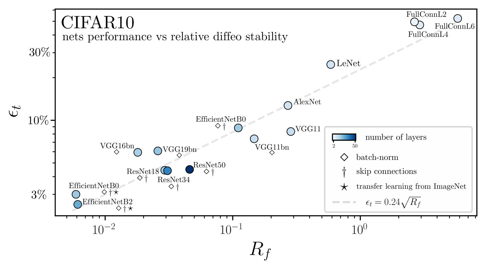
\(R_f = \frac{\mathbb{E}_{x,\tau}\|f(\tau(x))-f(x)\|^2}{\mathbb{E}_{x,\eta}\| f(x+\eta)-f(x)\|^2} \)
Hypothesis:
better nets are more stable to diffeo perturbations
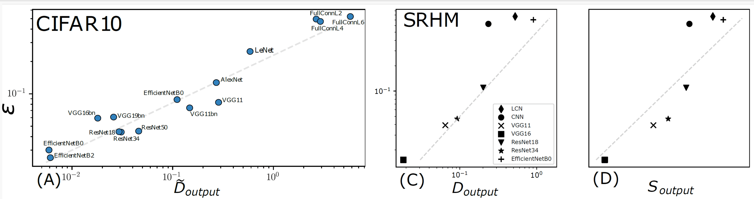
'Relative stability toward diffeomorphisms indicates performance in deep nets', NeurIPS 2021
Relative insensitivity to diffeomorphisms strongly correlates to performance!
+ Error
- Error
- Sensitive
+ Sensitive
'Relative stability toward diffeomorphisms indicates performance in deep nets', NeurIPS 2021
\(\textcolor{blue}{D_f \propto \mathbb{E}_{x,\tau}\|f(\tau(x))-f(x)\|^2} \)
\(\textcolor{green}{G_f \propto \mathbb{E}_{x,\eta}\| f(x+\eta)-f(x)\|^2}\)
with \(x\), \(x_1\) and \(x_2\) from test set
Performance correlates with stability to diffeo
\(R_f=\frac{D_f}{G_f}\)
\(R_f = \frac{\textcolor{blue}{\mathbb{E}_{x,\tau}\|f(\tau(x))-f(x)\|^2}}{\textcolor{green}{\mathbb{E}_{x,\eta}\| f(x+\eta)-f(x)\|^2}} \)
diffeomorphisms
random transformation
Performance correlates with sensitivity to noise
Questions:
- Why such a strong correlation between performance and sensitivity to diffeo exists?
- Which are the mechanisms learnt by CNNs which grant them insensitivity to diffeo?
Which operations give insensitivity to diffeo?
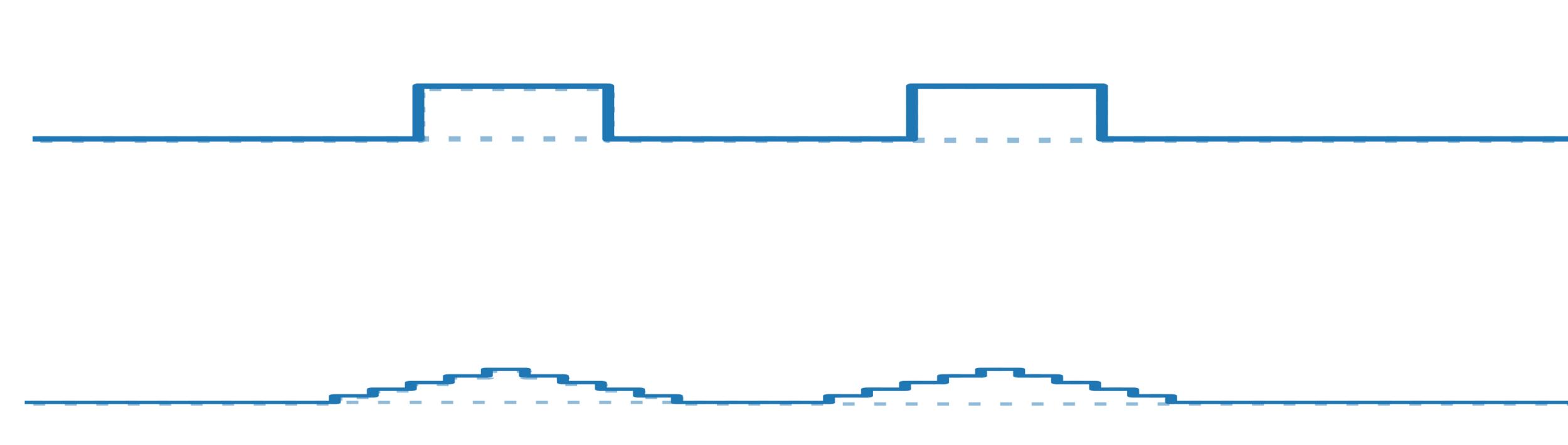
Spatial pooling
Channel pooling
Average pooling can be learned by making filters low pass
Channel pooling can be learned by properly adding filters together
- Reduce the resolution of the feature maps by aggregating pixel values
- Pooling across channels.
- Can give stability to any local transformation.
\(w\cdot x=\)
\(1.0\)
0.2
filters \(w\)
1
input \(x\)
0.2
\(1.0\)
1
rotated input

'How deep convolutional neural network lose spatial information with training',
[ICLR23 Workshop], [Machine Learning: Science and Technology 2023]
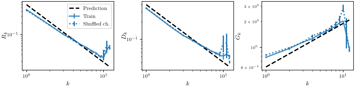
Both poolings are learnt
- \(R_k\) decreases in \(k\): both poolings are present (full lines).
- To disentangle the poolings, we shuffle inter-layer connections (dashed).
\(R_k = \frac{\mathbb{E}_{x,\tau}\|f_k(\tau(x))-f_k(x)\|^2}{\mathbb{E}_{x,\eta}\| f_k(x+\eta)-f_k(x)\|^2} \)
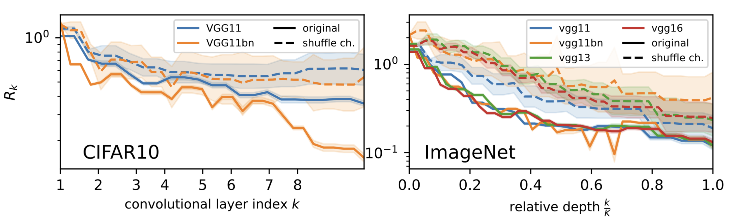
- Sensitive
+ Sensitive
- If only spatial pooling: the shuffled and original curves would overlap.
- If only channel pooling: the shuffled curves would be constant.
\(\rightarrow\) Neither the case: both poolings are learnt
We look at \(R_k\) of the representation \(f_k\) at layer \(k\).
- Spatial pooling plays a key role in reducing sensitivity to diffeomorphisms.
- To understand the consequences of this phenomenon, we use a simple model.
- It will capture why nets learn to become more sensitive to noise.
A simple Scale-Detection task
for spatial pooling
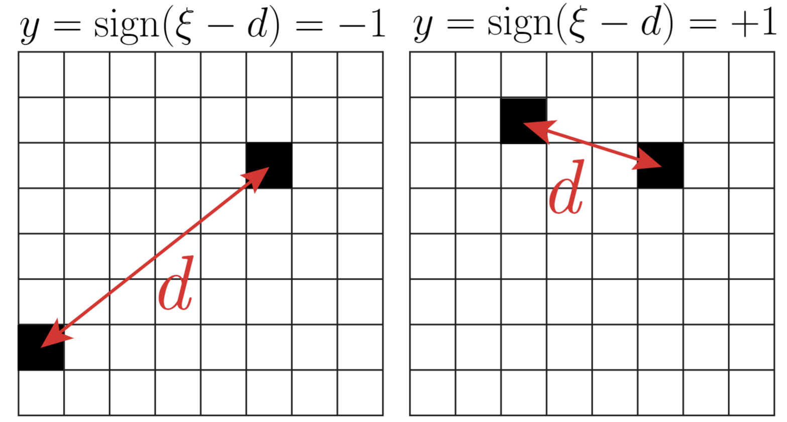
\(d\): distance between
active pixels
\(\xi\): characteristic scale
- Model where the exact positions of the features is not relevant
- Intuition: trained nets build spatial pooling solution up to scale \(\xi\) to solve the task
\(d<\xi\,\rightarrow\, y=-1\)
\(d>\xi\,\rightarrow\, y=1\)
Just spatial pooling is learnt
- Shuffling channels has no effect on the sensitivities \(\rightarrow\) Spatial pooling solution
- Our model captures the fact that while sensitivity to diffeo decreases, the sensitivity to noise increases
Why \(G_k\) increases?
\(R_k=\frac{D_k}{G_k}\)
\(\textcolor{black}{D_k \propto \mathbb{E}_{x,\tau}\|f_k(\tau(x))-f_k(x)\|^2} \)
\(G_k \propto \mathbb{E}_{x,\eta}\| f_k(x+\eta)-f_k(x)\|^2\)
Sensitivity to noise increseas layer by layer:
The positive noise piles up, affecting the representation more and more
How sensitivity to noise builds up in the net

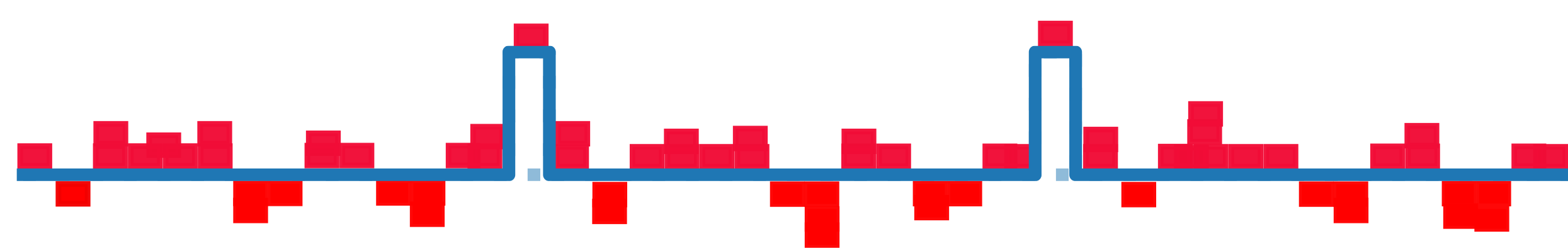
ReLU
\(x_i\sim\mathcal{N}(0,1),\) \(i\in\{1,...,N\}\)
\(\rightarrow\frac{1}{N}\sum_{i=1}^N x_i\approx 0\)
\(\rightarrow\frac{1}{N}\sum_{i=1}^N \textcolor{red}{|x_i|>0}\)
1/2 talk take-aways
- Two mechanisms are responsible for building representations insensitive to diffeomorphisms: spatial and channel pooling.
- Spatial pooling increases sensitivity to random noise.
- Seek to explain the correlation between performance and sensitivity to diffeo, using hierarchical models where information within the image is sparse.
Coming next
- Representations become increasingly better at discarding task-irrelevant information
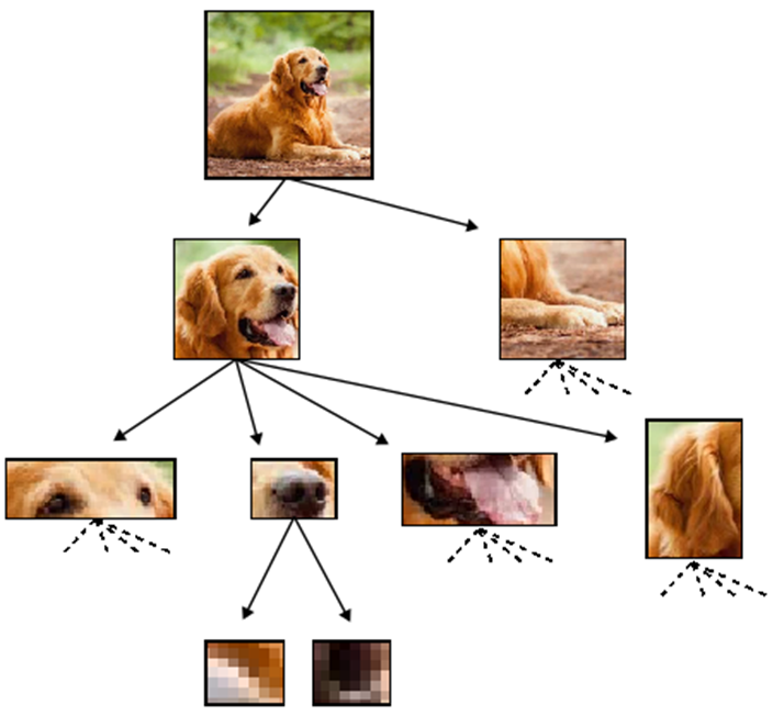
- Furthermore, the representations learn an hierarchy of concepts with increasing complexity with depth [e.g. edges \(\rightarrow\) abstract concepts]
Outline:
- Present a model where we can observe the same hierarchy of concepts
- Quantify how many training data are needed to learn (i) such hierarchy (ii) the task
- Later: connect with diffeomorphisms
Key limitation of RHM:
- Real images: invariance to diffeo
- RHM: moving one pixel will likely change the image label.
To overcome it:
We introduce a model where the features are sparse and hierarchically structured.
- We show that diffeo and synonyms are learnt together with the task, with a number of training points \(P^*\) polynomial in the dimension.
- Understanding: local reconstruction of the hierarchy (key to learn the task) happens at each equivalent location, yielding invariance to smooth transformations.
How about weight-sharing (CNNs)?
\(P^*\sim\textcolor{blue}{ (s_0+1)^2} n_c m^L\)
Task
Sensitivities
- The signal is exponentially diluted layer by layer: \(\sim1/(s_0+1)^{L}\)
- The same weight looks at a number of locations \([s(s_0+1)]^{L-1}\) exponentially large in \(L\)
\(\Rightarrow\) To recover the synonyms, a number of training points of order \(P^*_0\) is needed, up to a constant in \(L\), which we observe being \((s_0+1)^2\).
Why CNNs have this \(P^*\)?
\(P^*_{\text{CNN}}\sim F^{-2/L} [n_c m^L]\)
\(P^*_{\text{LCN}}\sim \frac{1}{F}s^{L/2}[ n_c m^L]\)
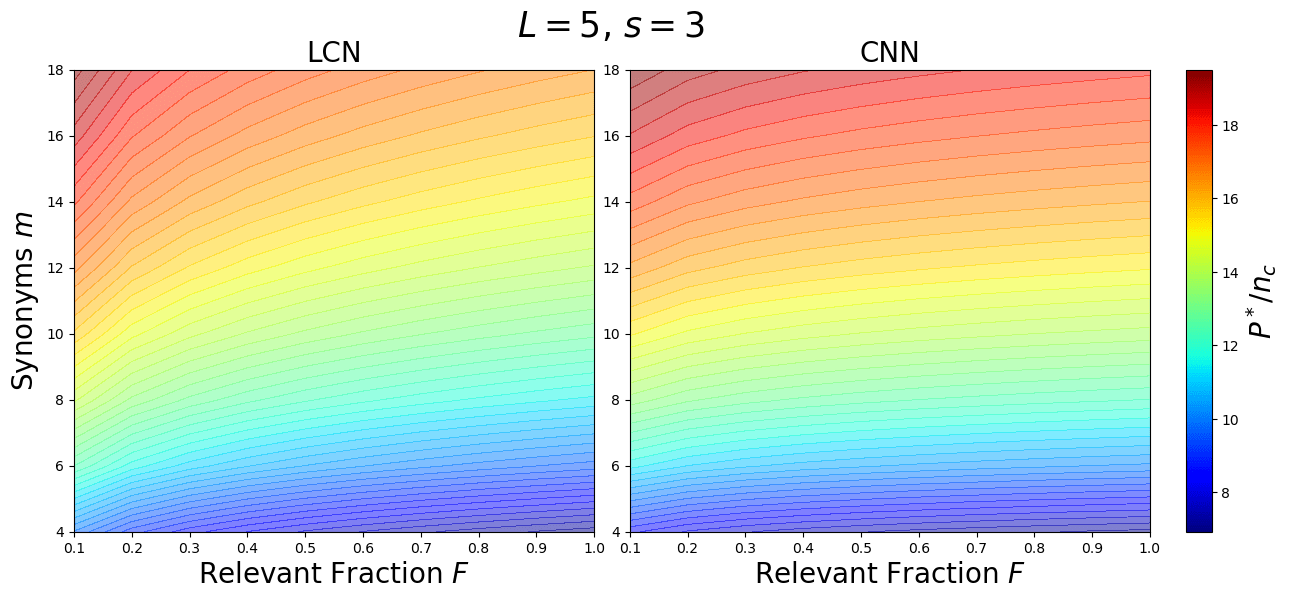
\(F\): image relevant fraction
- Look whether also real networks trained on real data learn synonymic insensitivity and diffeo insensitivity at the same time as they learn the task.
Future directions
Thank you!
Image by [Kawar, Zada et al. 2023]
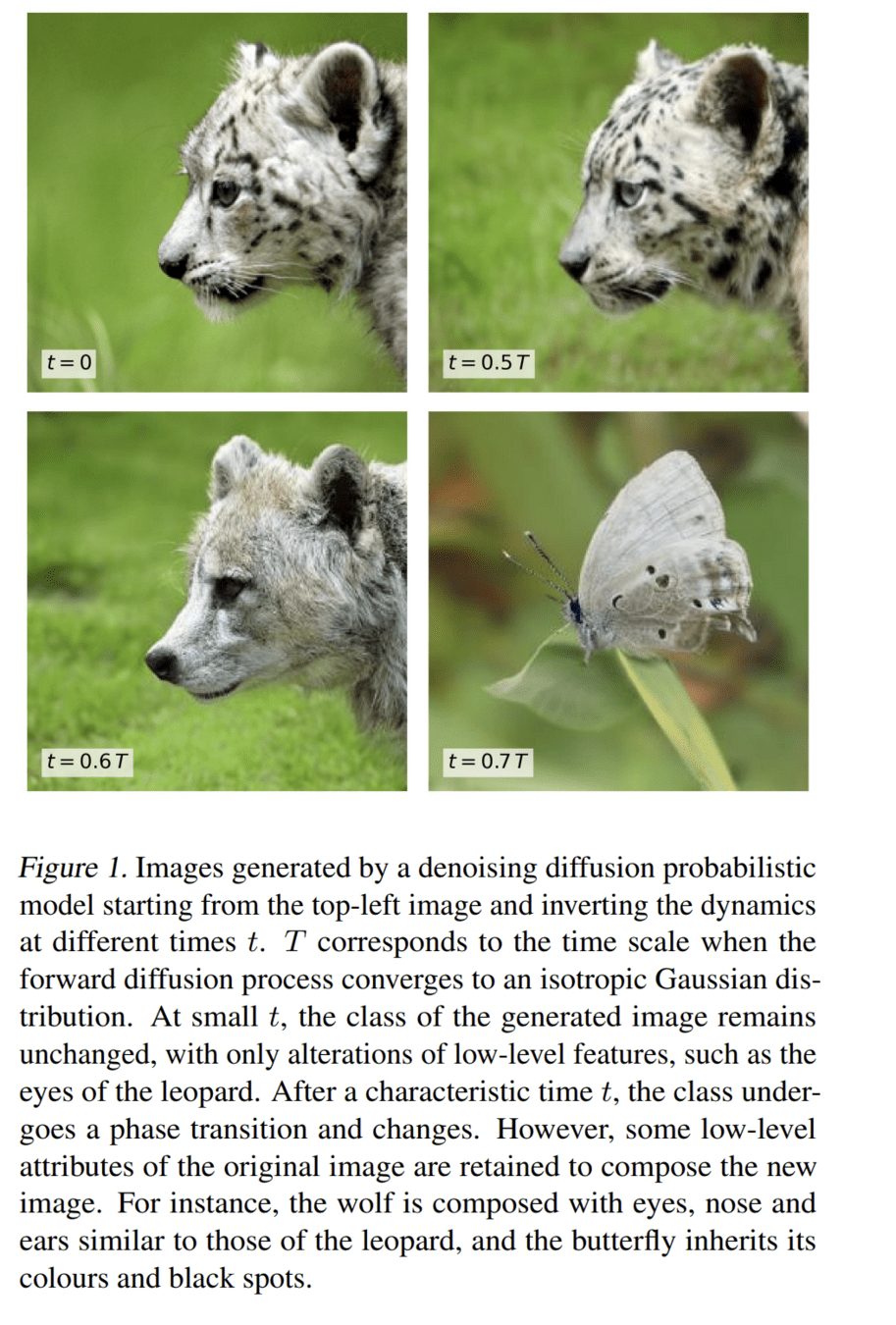
- We want to test also the following hypothesis: the best networks are the ones that become more insensitive to diffeomorphisms and synonyms.
- To test that, we need images where features at different levels of the hierarchy are modified. We plan to get them with diffusion.
- language!!! general properties of data!!
- multi modal model, same structure for text and vision
Which net do we use?
We consider a different version of a Convolutional Neural Network (CNN) without weight sharing
Standard CNN:
- local
- weight sharing
Locally Connected Network (LCN):
- local
weight sharing
- We take a 2-layer LCN, trained on the sparse hierarchical dataset (with \(v=m\) and \(L=2\)) with \(P\) training points;
- We apply either synonyms exchange or diffeo at the first level of the input data;
- We check whether the second net layer is sensitive to these transformations.
Testing synonymic and diffeo sensitivity
\( \textcolor{blue}{P_1}\): synonymic exchange at layer 1
\( \textcolor{blue}{S_{2, 1} \propto \langle\|f_{2}(x) - f_{2}(P_1 x)\|^2 \rangle_{x, P_1}}\)
Learning the task correlates with:
- Learning the synonymic equivalence
- Learning the diffeo stability
Synonymic and diffeo sensitivity
emerge at the same time
Is this observation robust? How many training data?
How many training data for LCNs?
To learn the task:
\(P^*\sim\textcolor{blue}{ (s_0+1)^L} n_c m^L\)
How many training data for LCNs?
- Without sparsity (\(s_0=0\)) the number of training points to learn the synonyms and hence the task is \(P^*_0\sim n_c m^L\)
- With sparsity, for most of the data, a local weight does not see anything.
\(\Rightarrow\)To recover the synonyms and then solve the task,
it is then necessary to see many more data:
\(P^*_{\text{LCN}}\sim (s_0+1)^L P^*_0\)
\(s_0=1\)
Probability to see a signal in a given location:
\(p=\frac{1}{(s_0+1)^L}\)
\(\Rightarrow\) change polynomial in \(d=(s(s0+1))^L\)
Take-aways
- Stability to diffeo and invariance to synonyms are learnt together, precisely where test error drops.
- If a network reconstructs the hierarchical task by leveraging local feature-label correlations, then it extends this capability at each equivalent location, yielding invariance to diffeo.
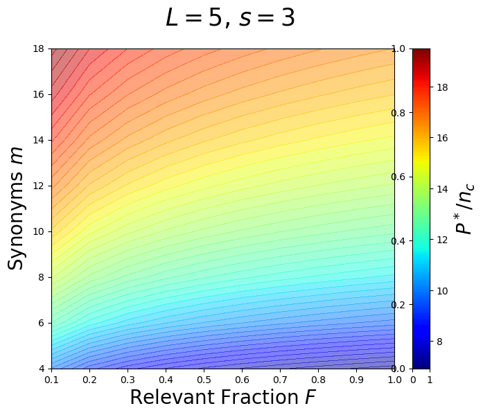
- Phase diagram for sample complexity for LCNs.
\(P^*_{\text{LCN}}\sim \frac{1}{F}s^{L/2}[ n_c m^L]\)
\(F\): image relevant fraction