Machine Learning & Advanced Analytics for Biomedicine
BMI 633
Ishanu Chattopadhyay
Assistant Professor of Biomedical Informatics and Computer Science

ishanu_ch@uky.edu

Machine Learning & Advanced Analytics for Biomedicine
Machine Learning & Advanced Analytics for Biomedicine
What is Machine Learning
Learning from machines?
Learning with the help of computers?
Modeling data?
Regression?
data -> (intelligent) automated analysis -> actionable insights
How is Machine Learning different from...
Statistics
AI
Data Mining
Deep Learning
How is Machine Learning different from...
"Machine learning is essentially a form of applied statistics”
“Machine learning is statistics scaled up to big data”
“Machine learning is Statistics minus any checking of models and assumptions.”
“I don’t know what Machine Learning will look like in ten years, but whatever it is I’m sure Statisticians will be whining that they did it earlier and better.”
Approach to a problem differs between mathematicians, statisticians & ML-experts
- Central Limit Theorem
- Measure Theory
- Stochastic Processes
- Linear Regression
- General Linear Models
- What is the "correct" statistical model for a problem/process ?
- Often interest is "describing" data already observed
- No model is correct.
- The useful ones predict correctly more often than others
- ONLY interested in how well a model works on unseen data
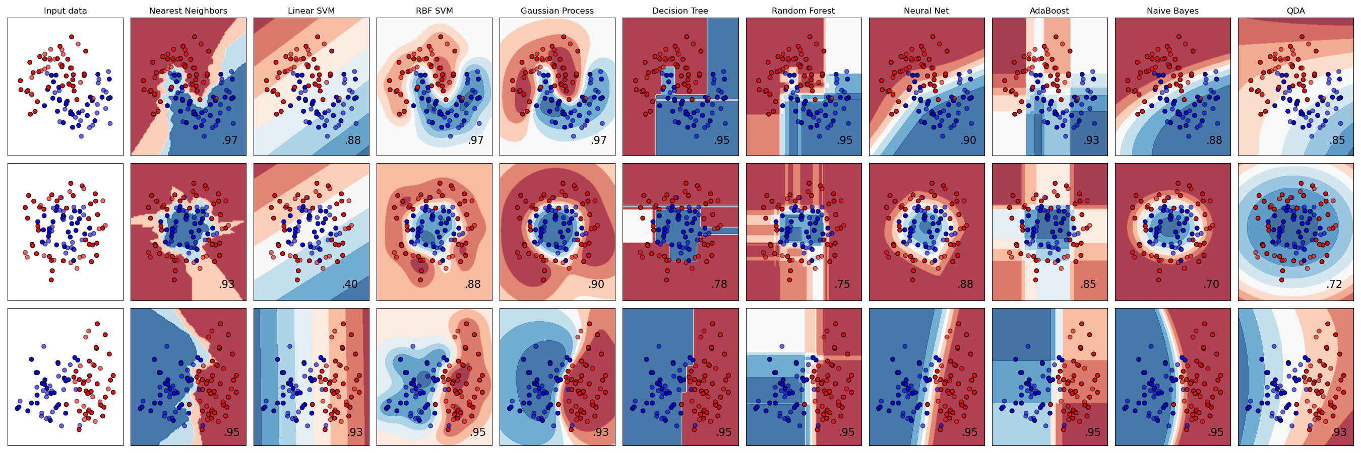
Decision Surfaces with Different Classification Algorithms
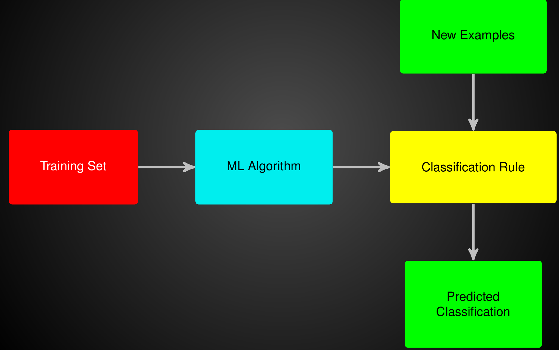
How Do We Teach Machines To..

Is there any good reason to assume that data that you have not seen yet will share any properties with data you have already seen?
ML Applications in Bio-medicine
Uncharted Possibilities
- Predicting future disease
- Optimizing interventions
- Discovering unknown mechanisms
- A new paradigm of scientific discovery
- At-scale pattern discovery impossible otherwise
Data
Knowledge
Towards a grand unified theory of data
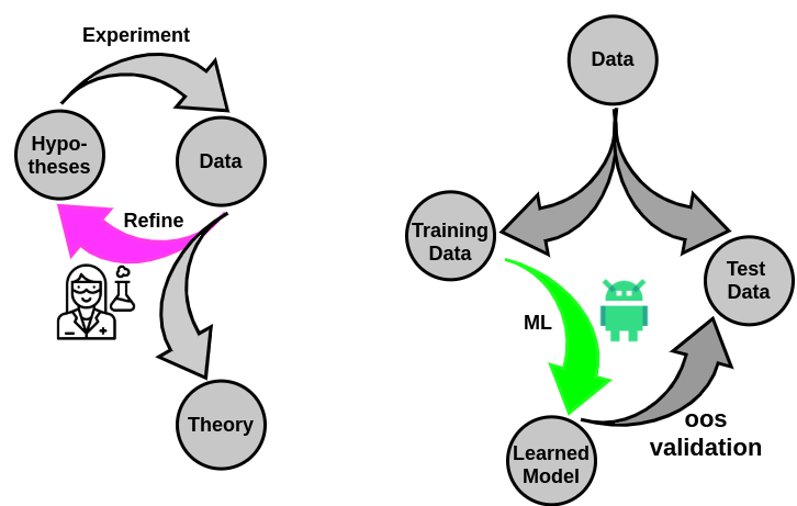
lots of data!

Classical Science
The age of data

Data


Insight
scientific knowledge
Clinical Decisions
social theory

Lets get down to the basics...
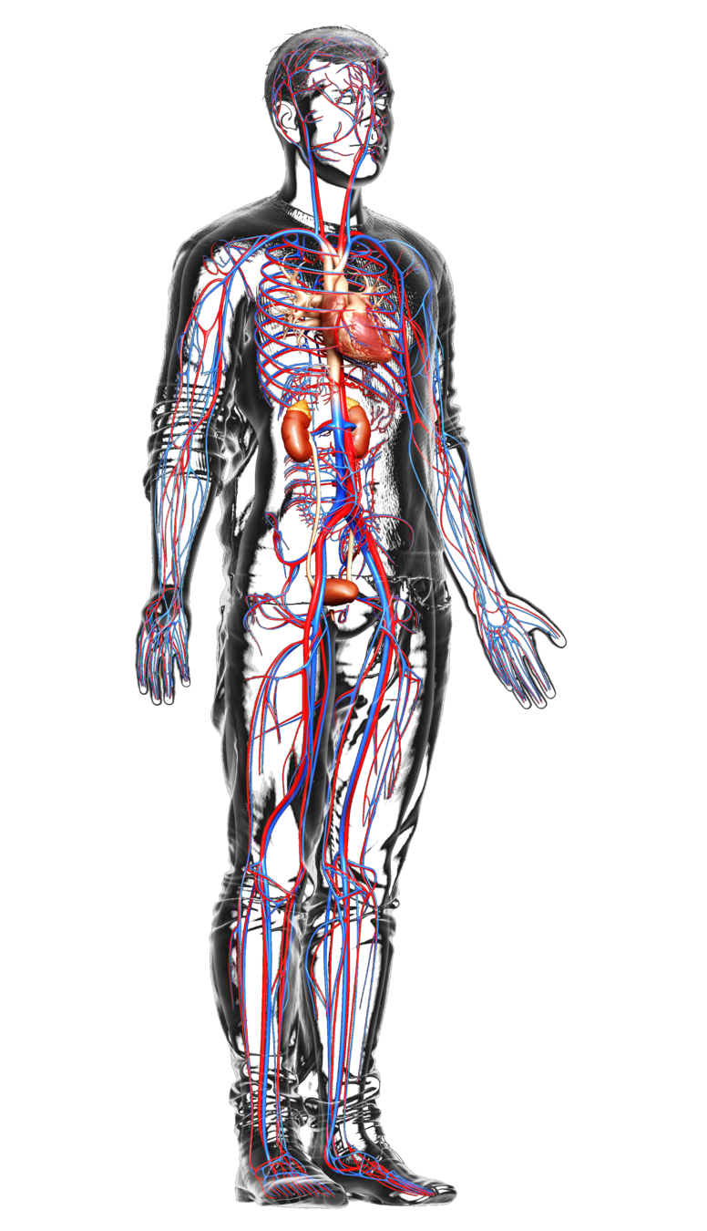
Diagnostic Tests for Diseases
- Risk Factors
- Past Diagnoses
- Laboratory Tests
- Questionnaire
- Familial Risks
- Life Events
Does the patient have the disorder?
Not Always Obvious
autism
dementia
Diagnostic Tests for Diseases
- Risk Factors
- Past Diagnoses
- Laboratory Tests
- Questionnaire
- Familial Risks
- Life Events
Does the patient have risk of the disorder ?
Not Always Obvious
autism
dementia
How do we quantify risk?
How do we map risk to severity?
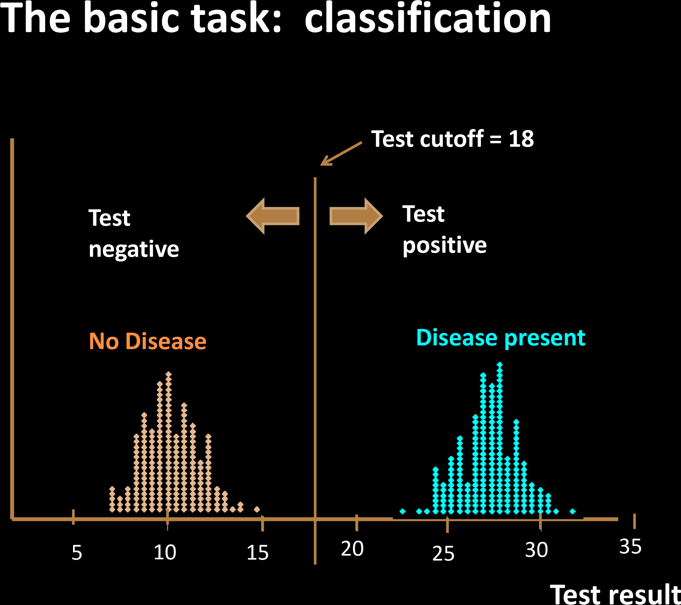
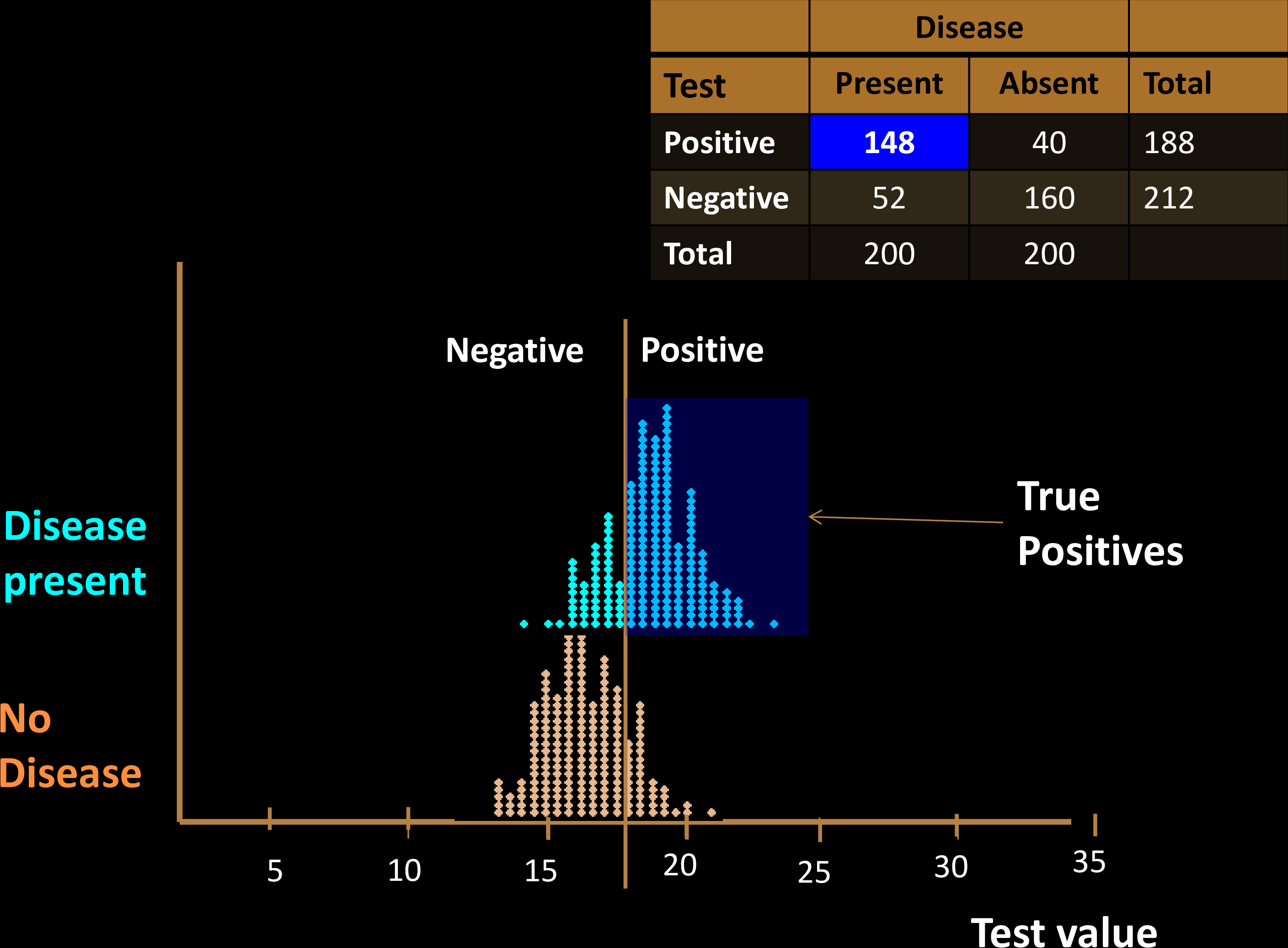
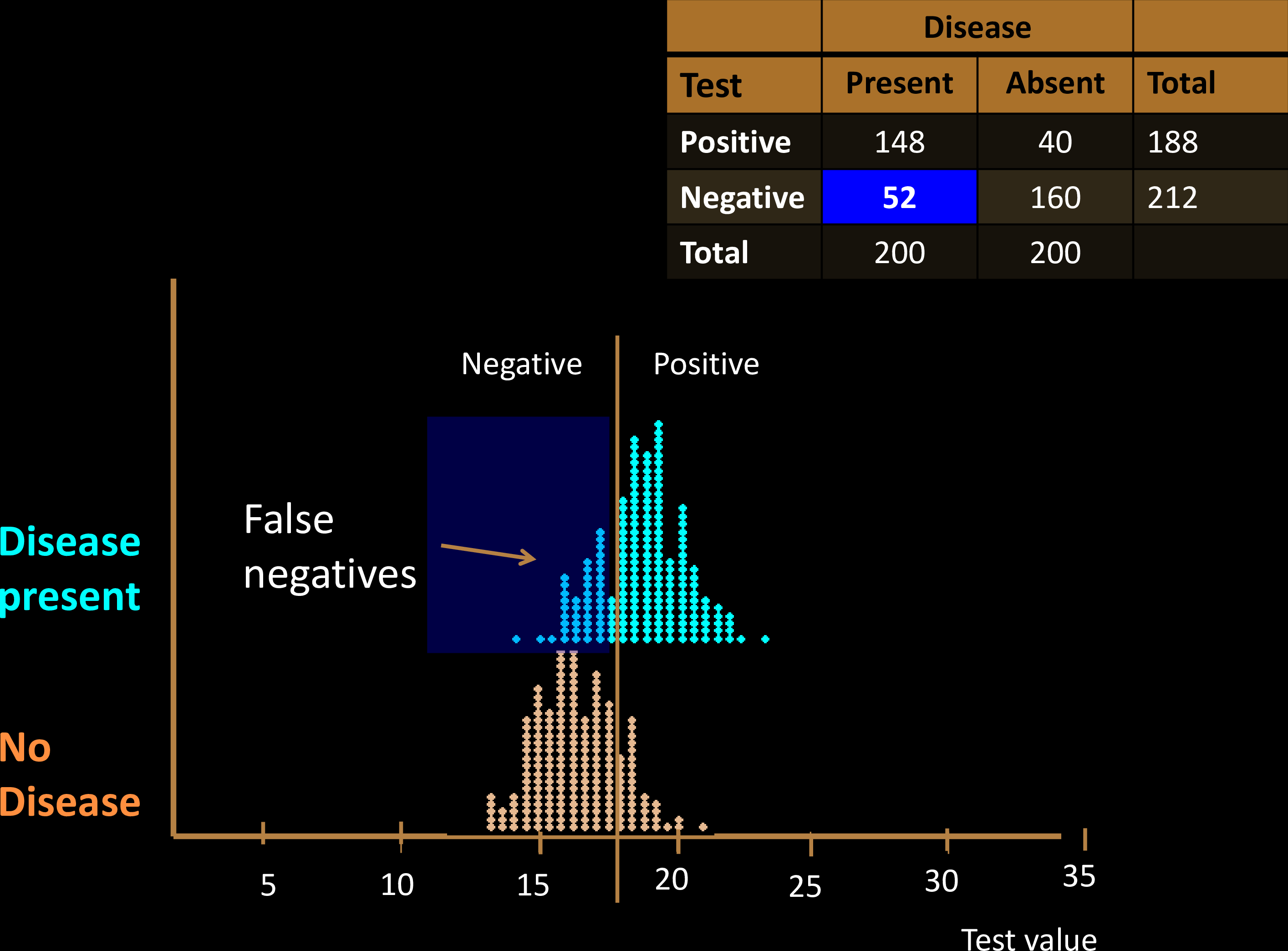
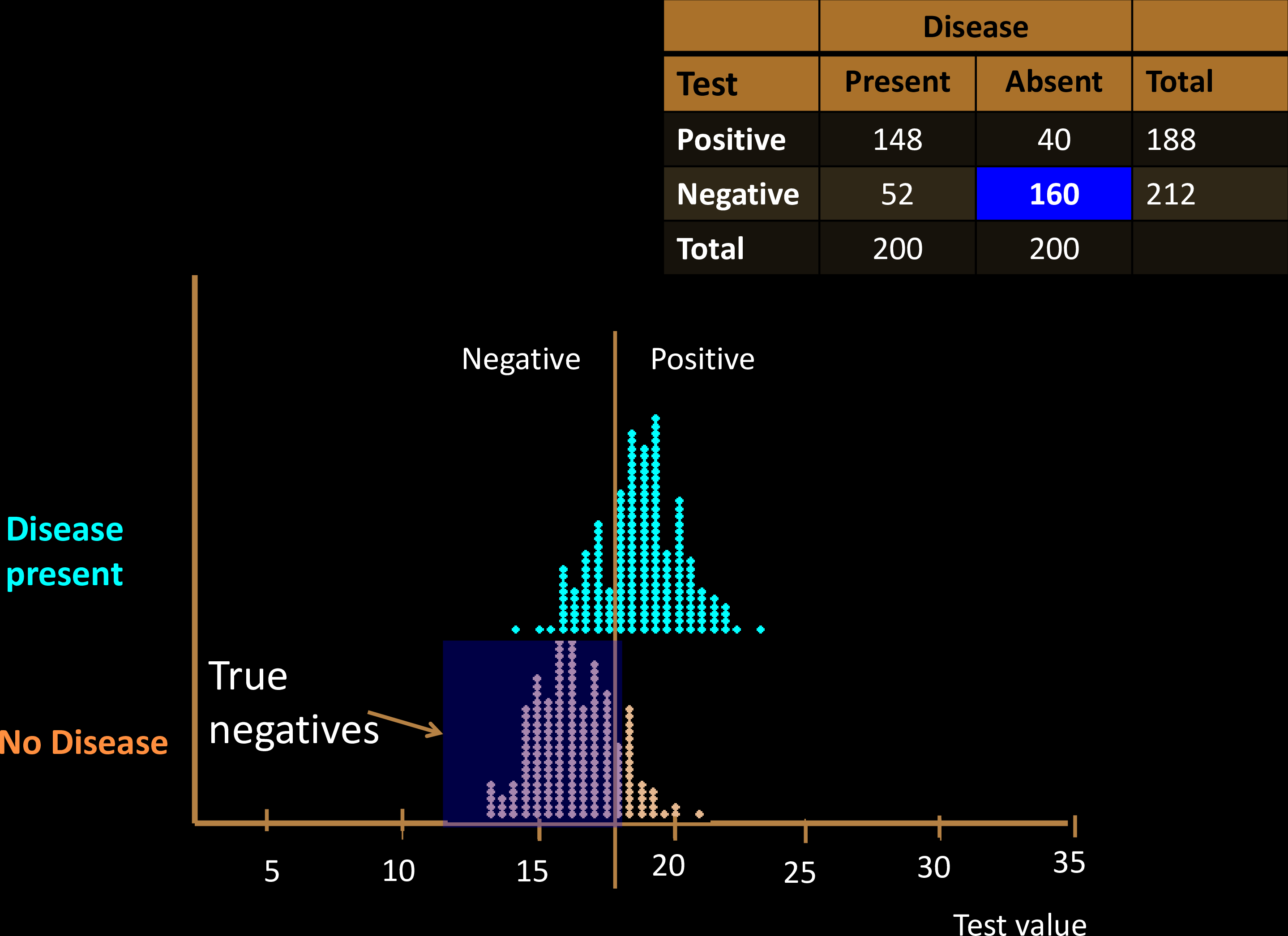
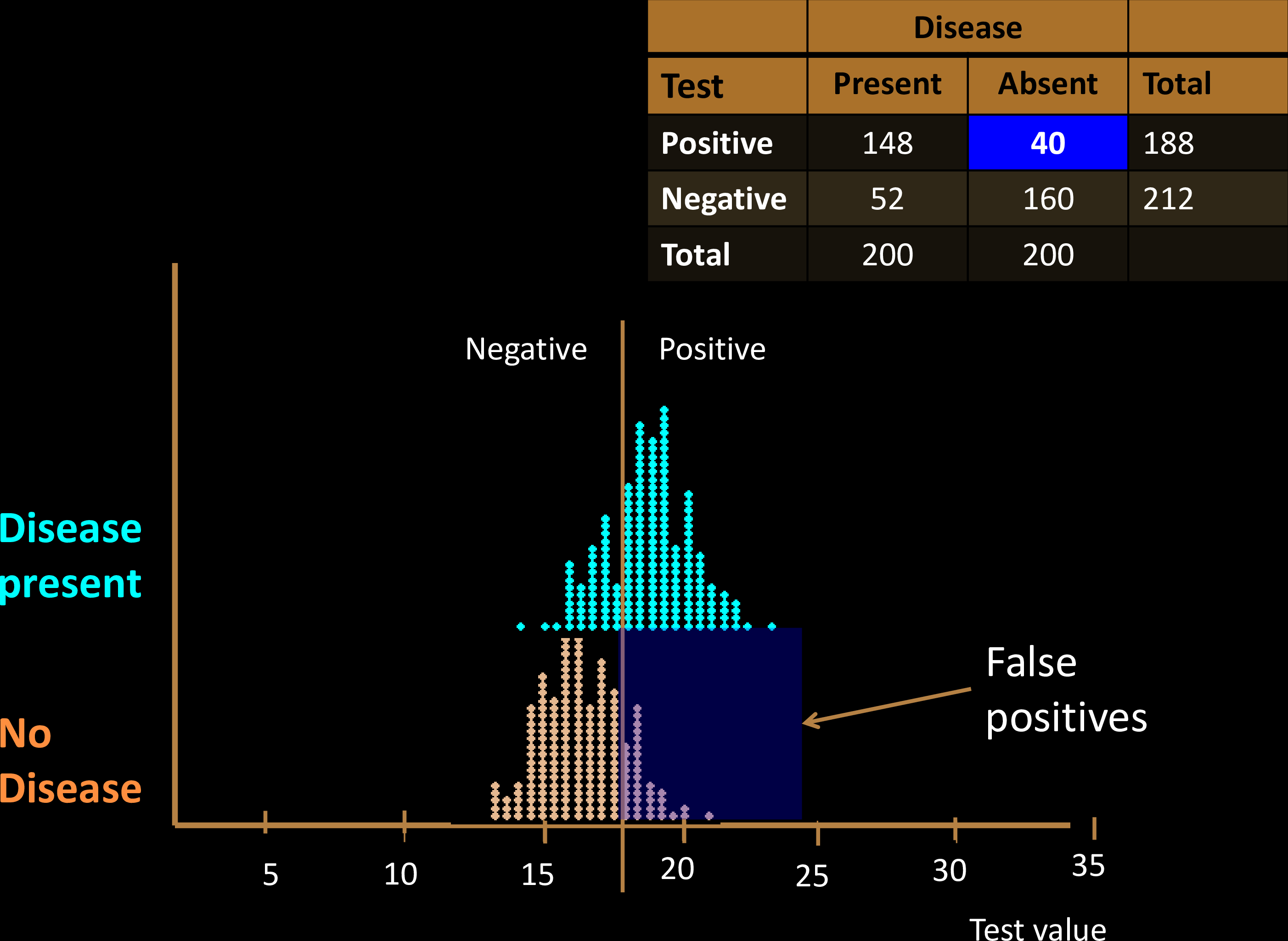
Diagnostic Tests
Diagnostic Tests
Diagnostic Tests
Diagnostic Tests
Diagnostic Tests
Diagnostic Tests
Diagnostic Tests
Diagnostic Tests
Diagnostic Tests
Diagnostic Tests
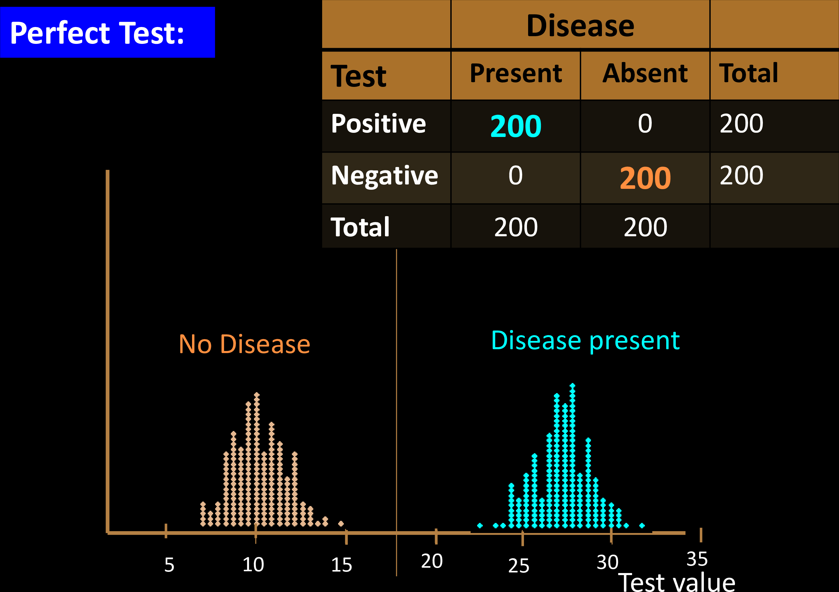
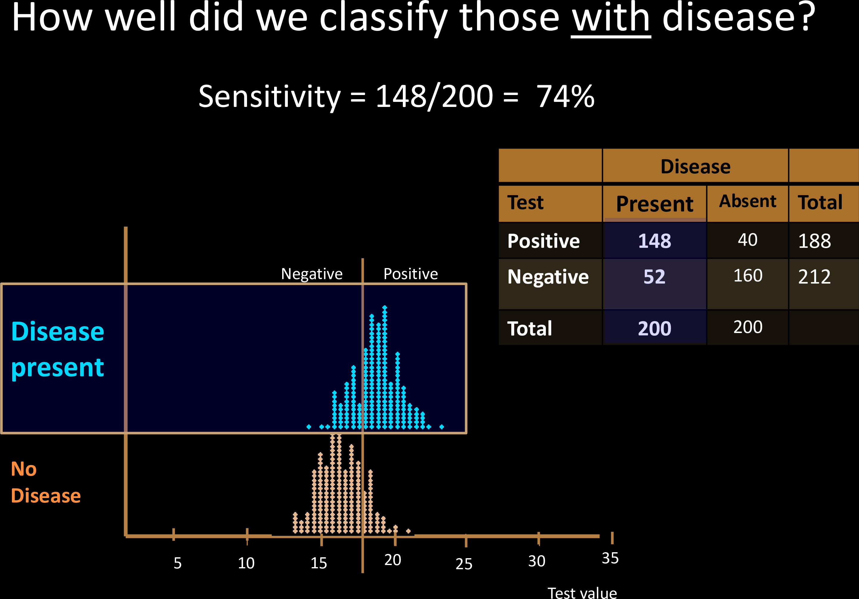
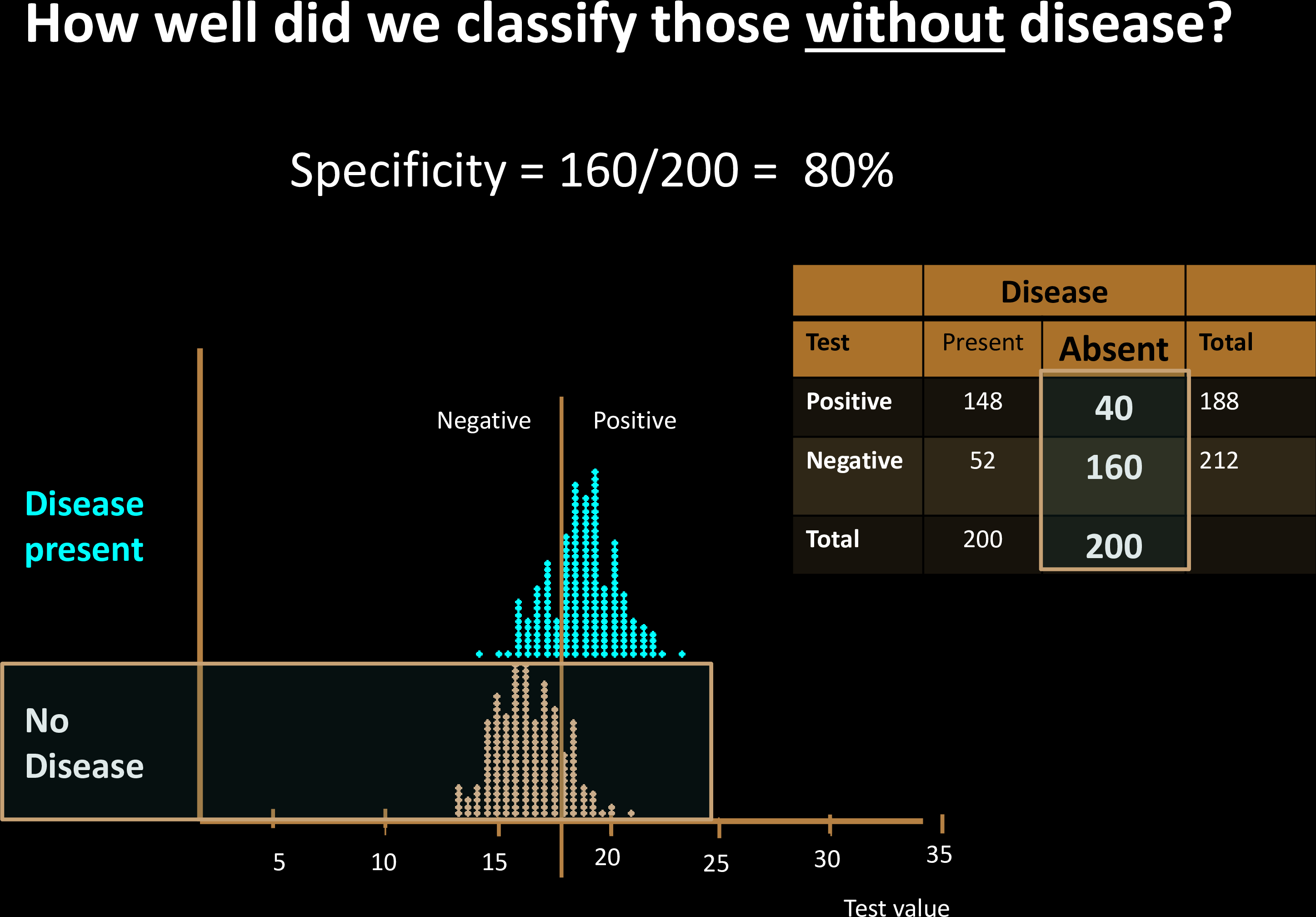
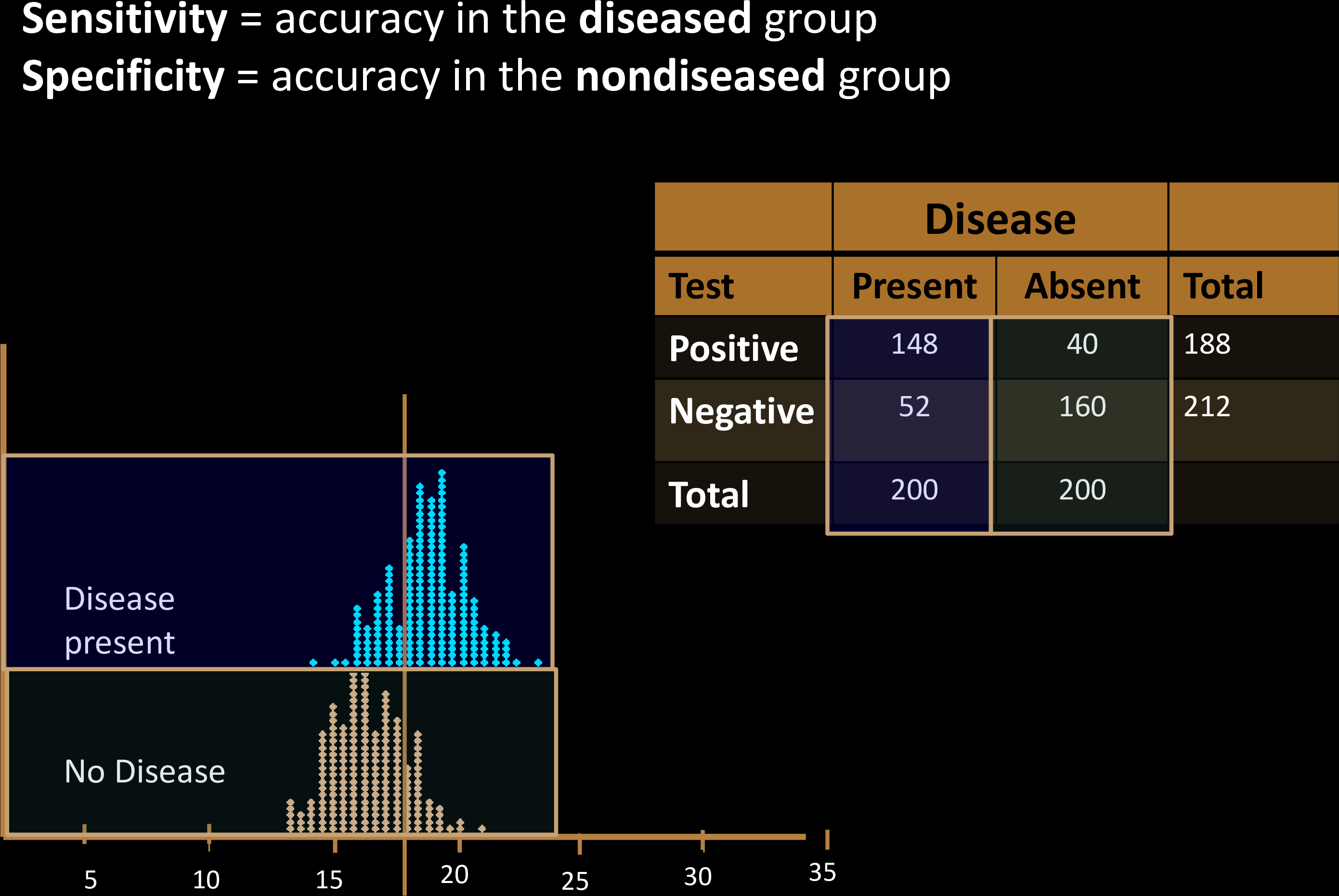
Sensitivity & Specificity
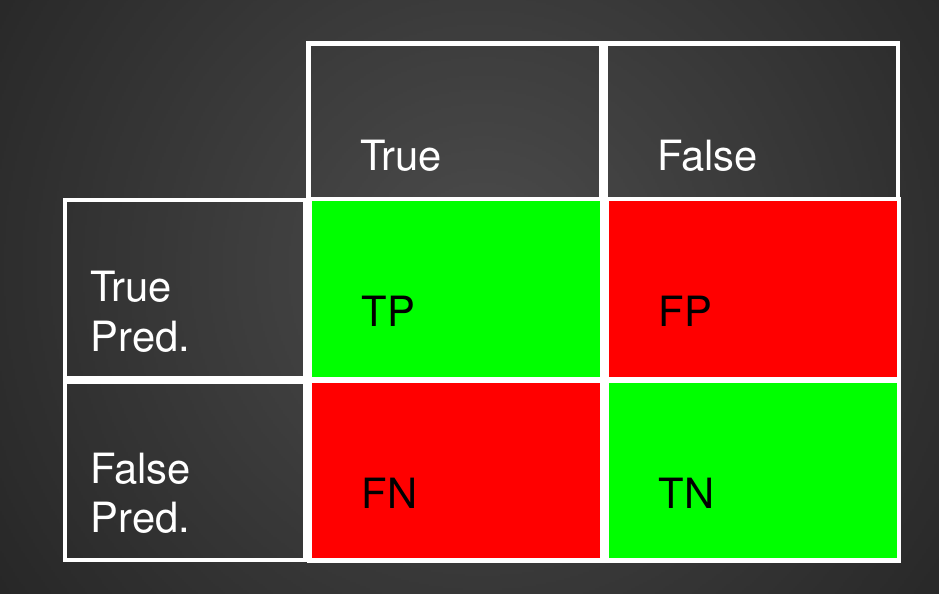
Confusion Matrix with 2 classes
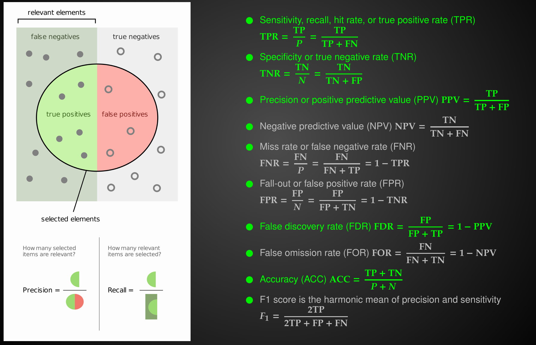
Performance Metrics
Relationships between Performance Metrics
Relationships between Performance Metrics
Relationships between Performance Metrics
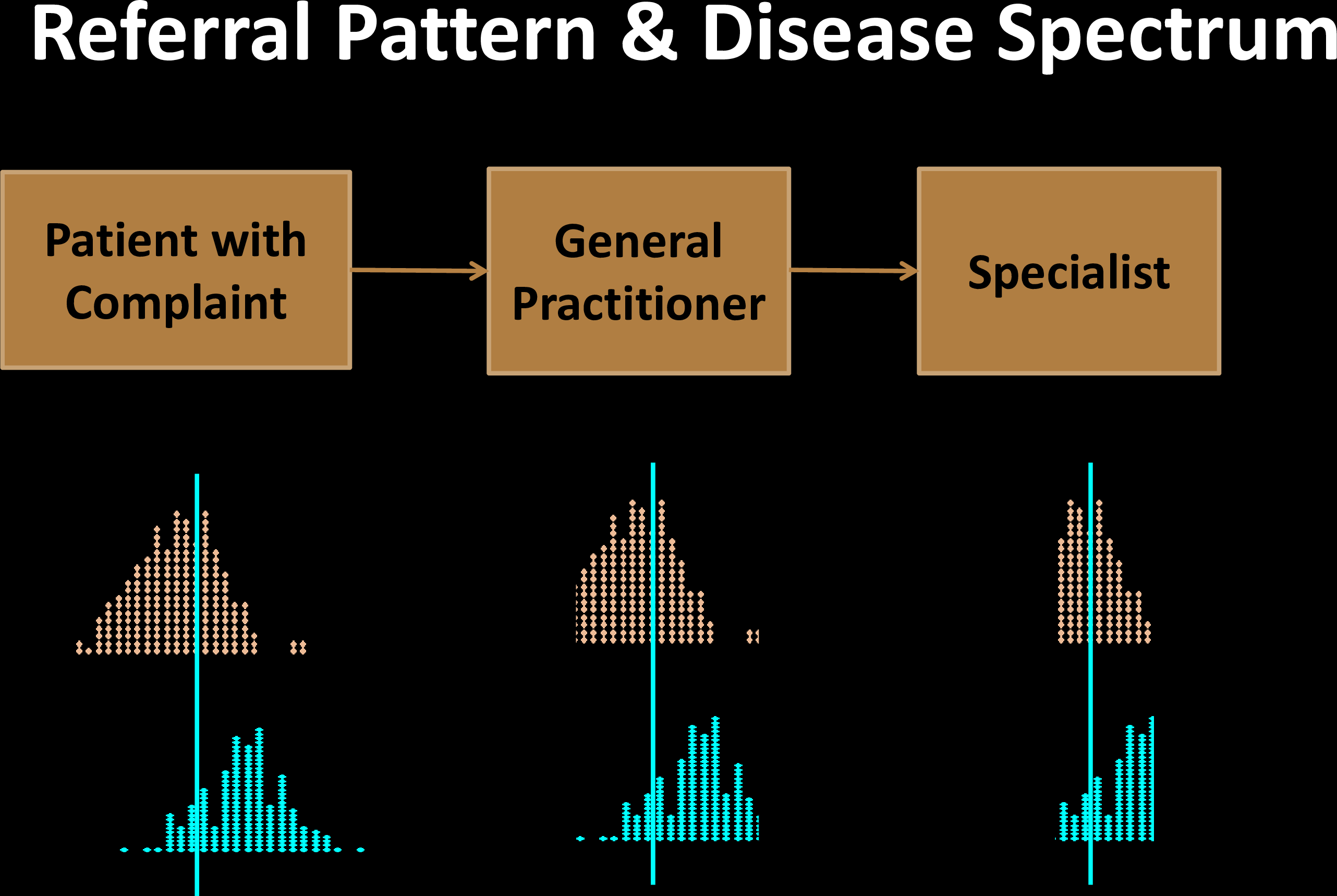
prevalence is intrinsic property of the disease
Relationships between Performance Metrics
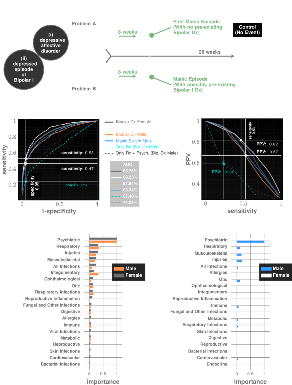
Manic Episode with no Bipolar history
prevalence: ~10%
Relationships between Performance Metrics
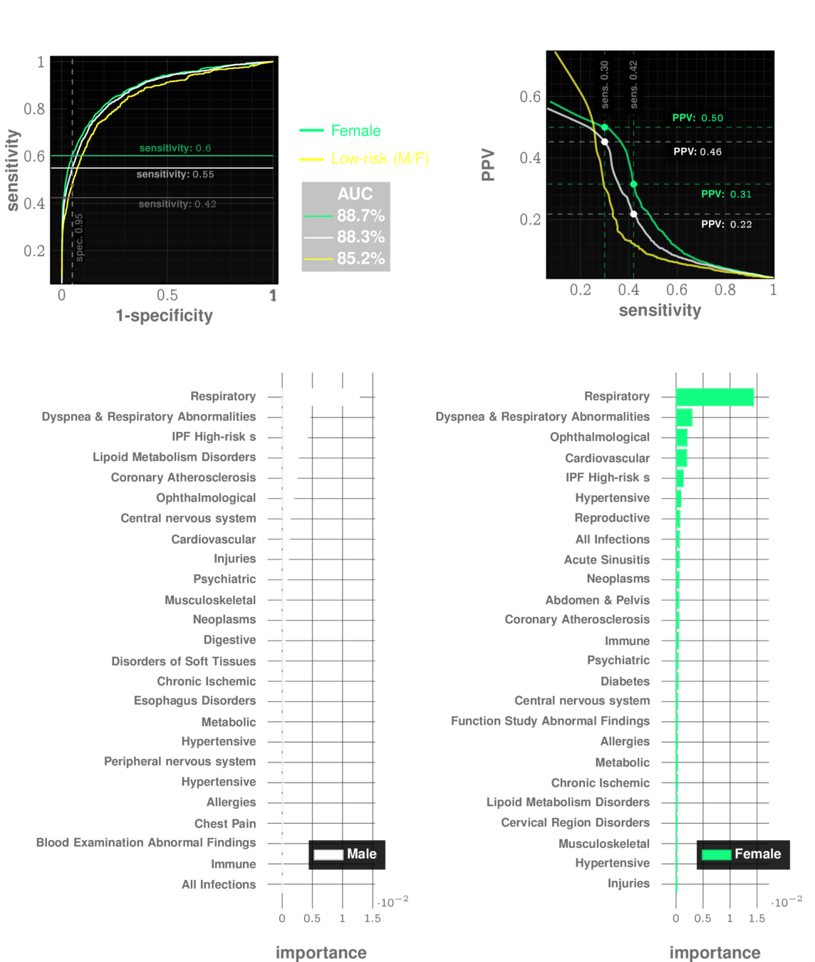
Idiopathic Pulmonary Fibrosis
prevalence: ~0.5%
Relationships between Performance Metrics
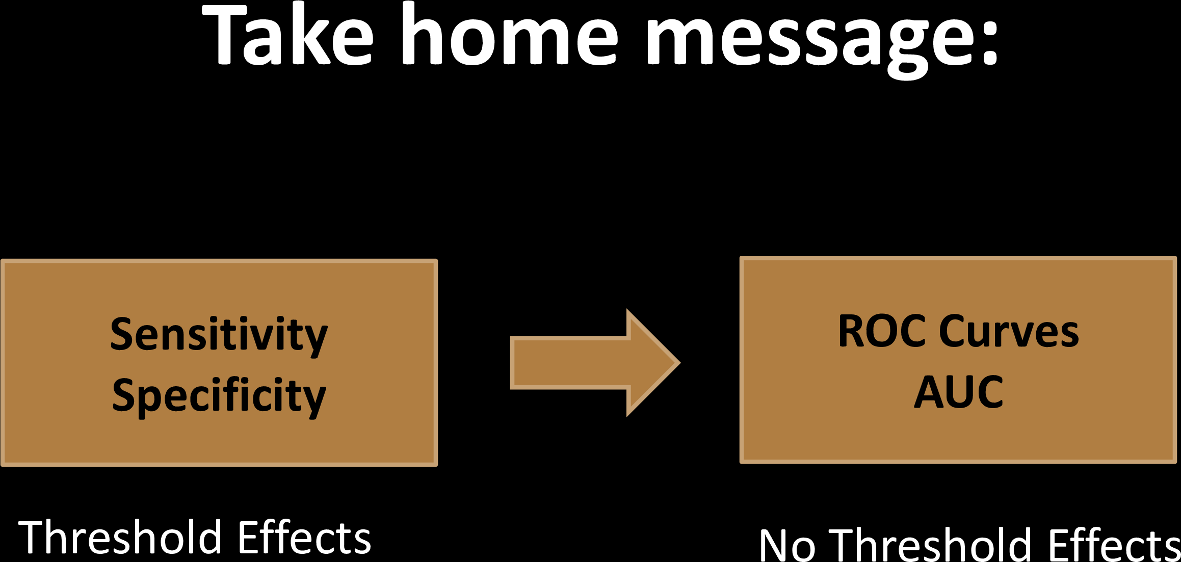
The decision threshold is upto us to decide
Impacts sensitivity & specificity
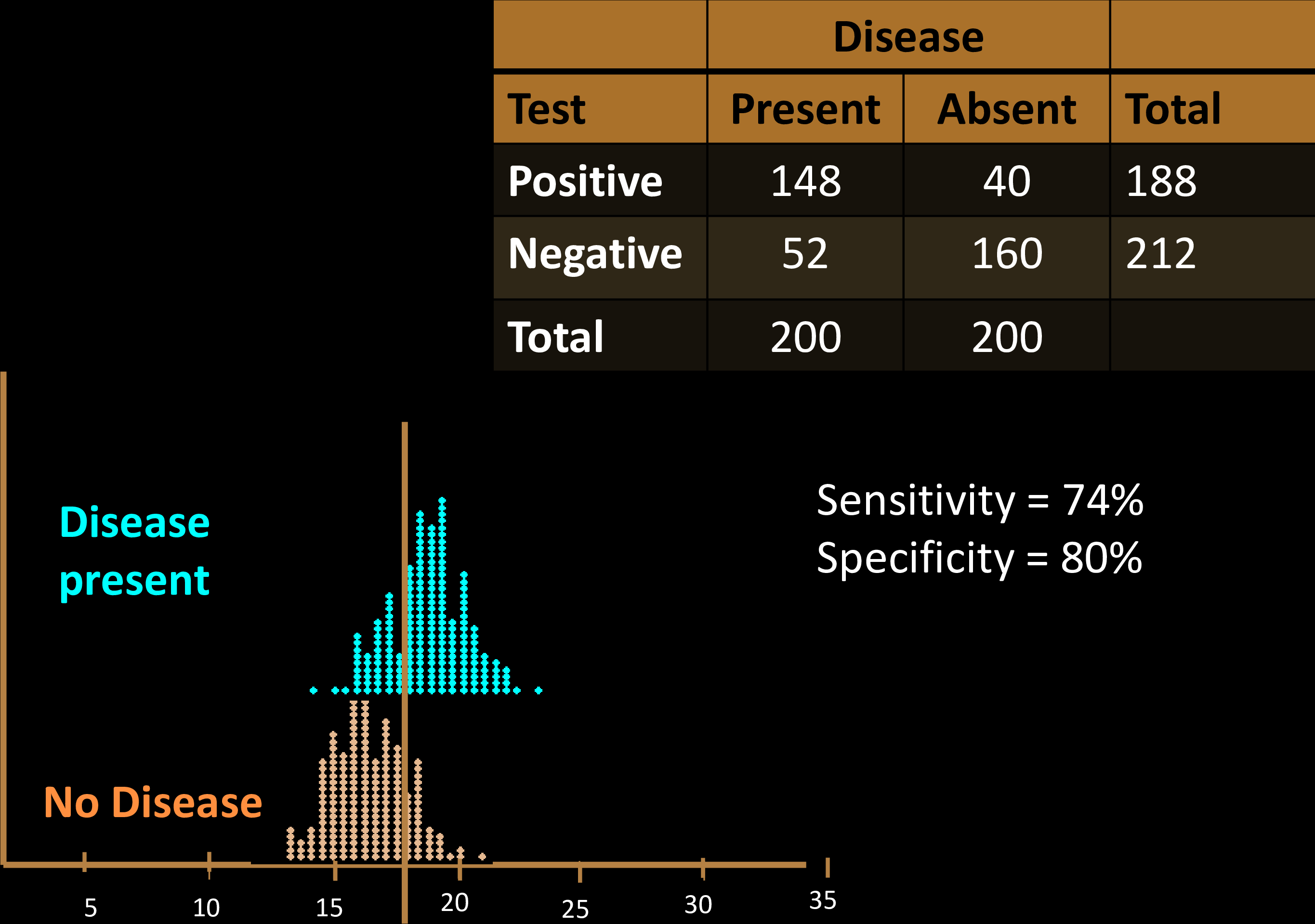
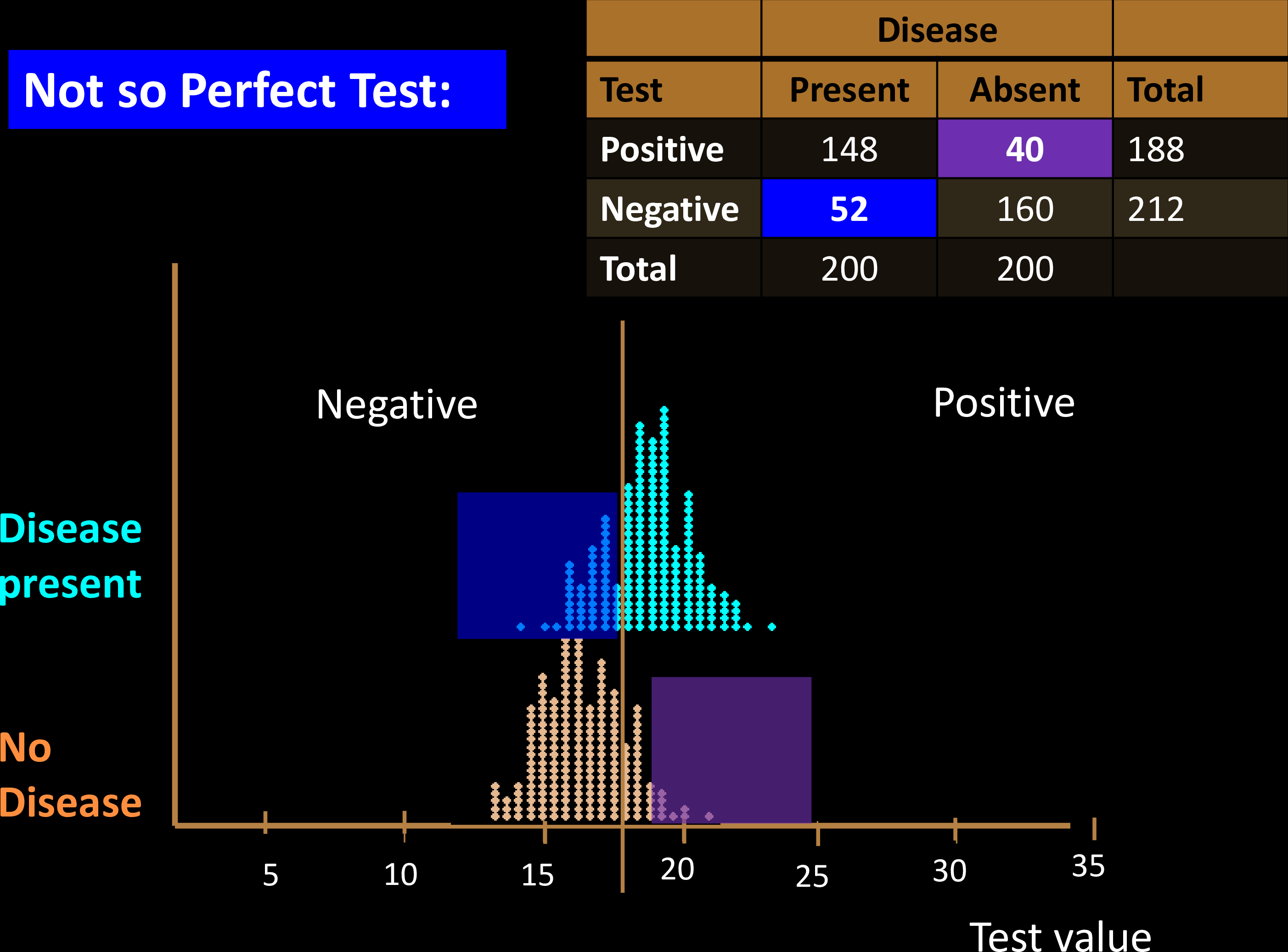
Sensitivity Specificity Tradeoff
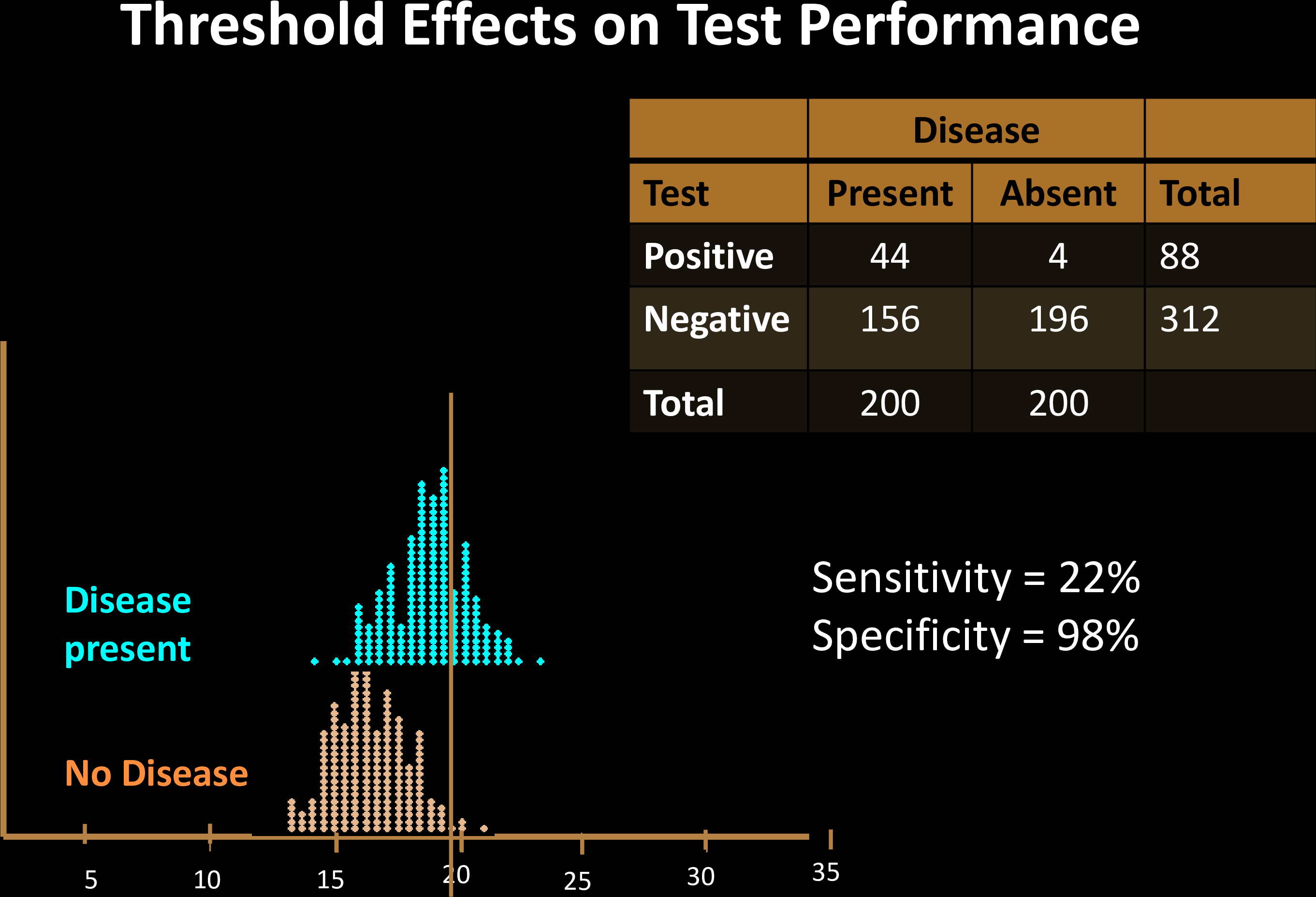
Sensitivity Specificity Tradeoff
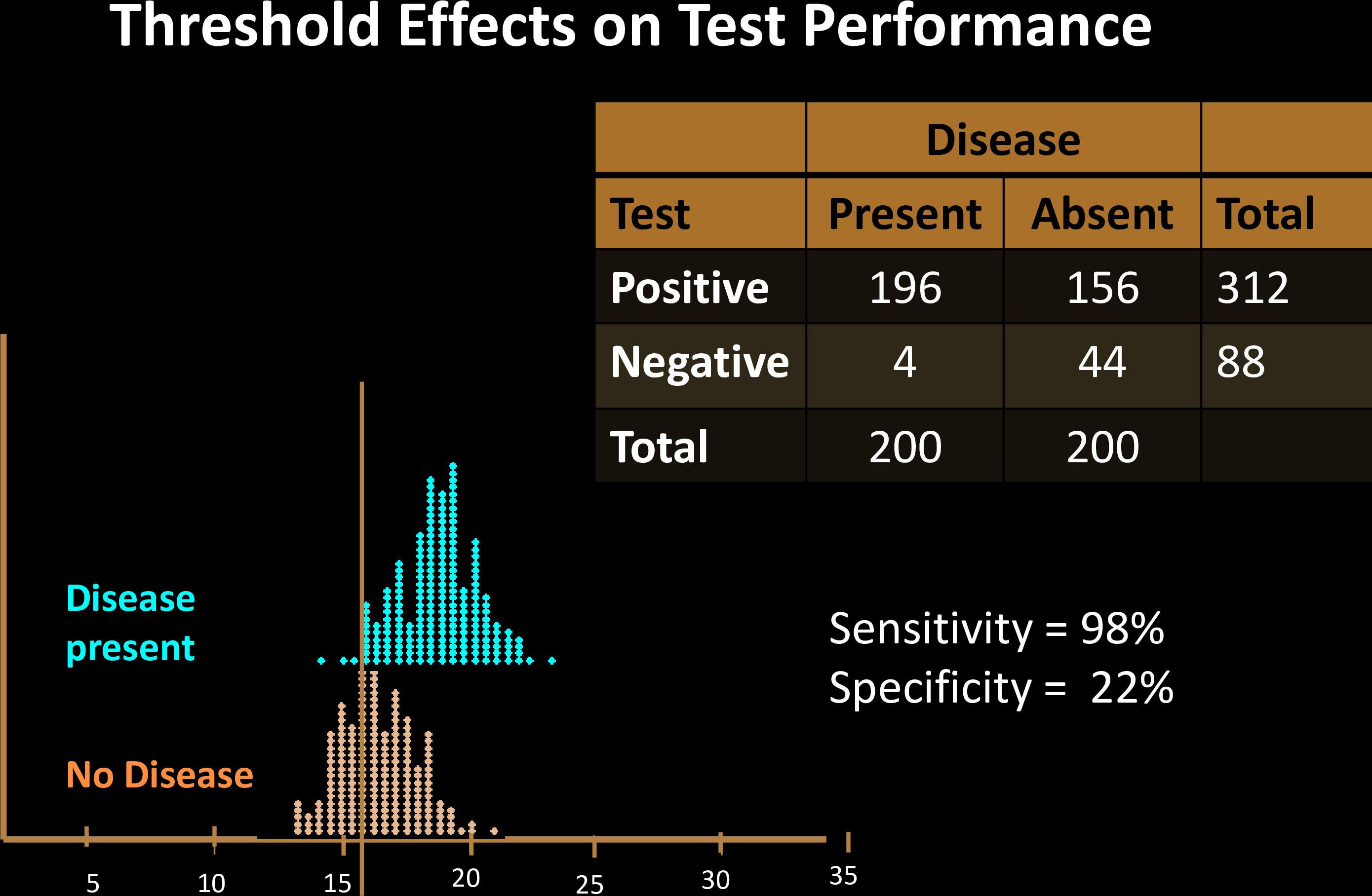
Sensitivity Specificity Tradeoff
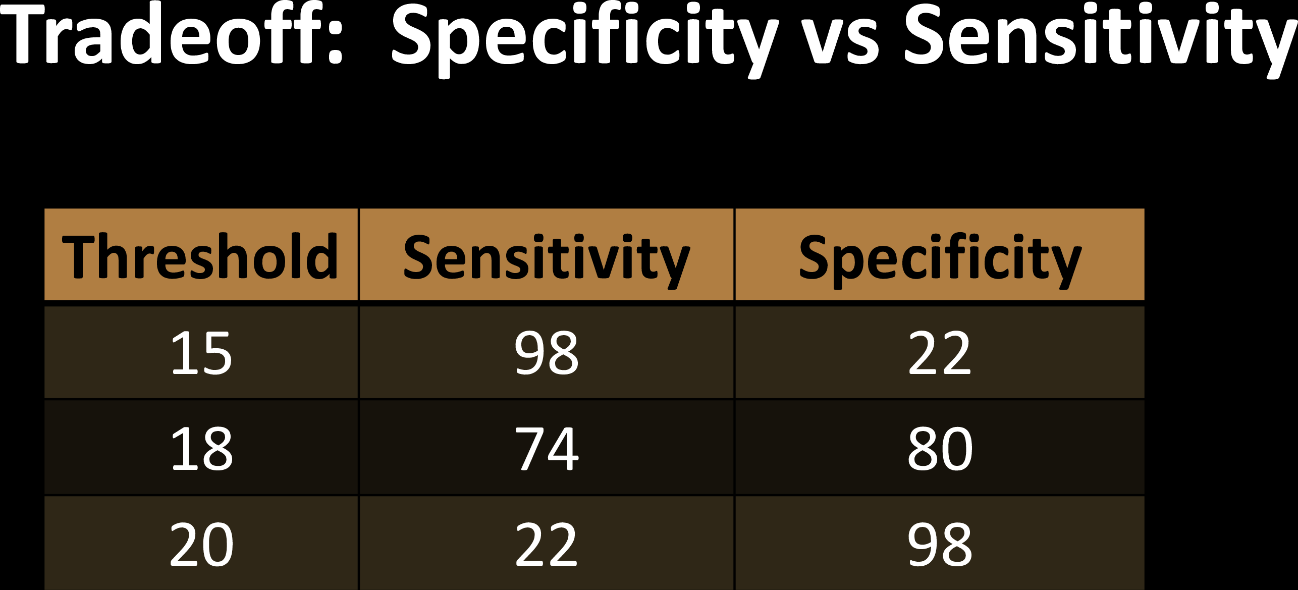
Sensitivity Specificity Tradeoff
Each choice of a threshold produces a different test
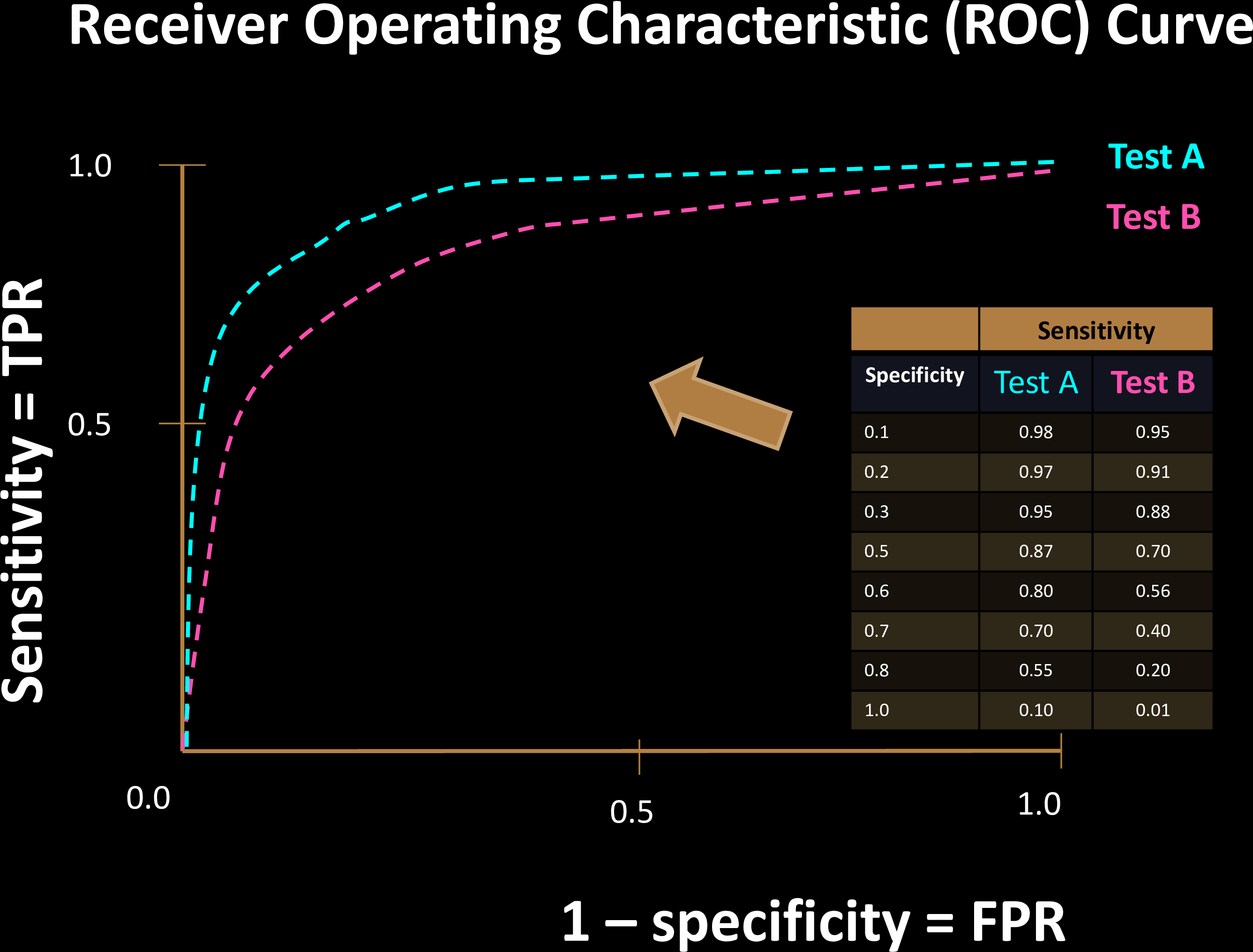
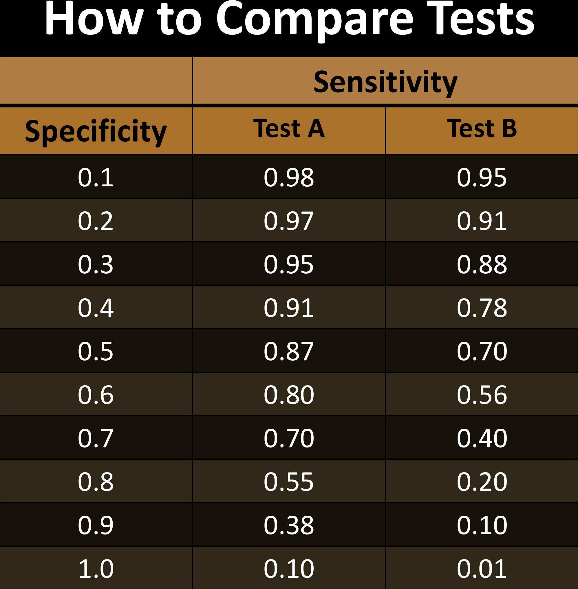
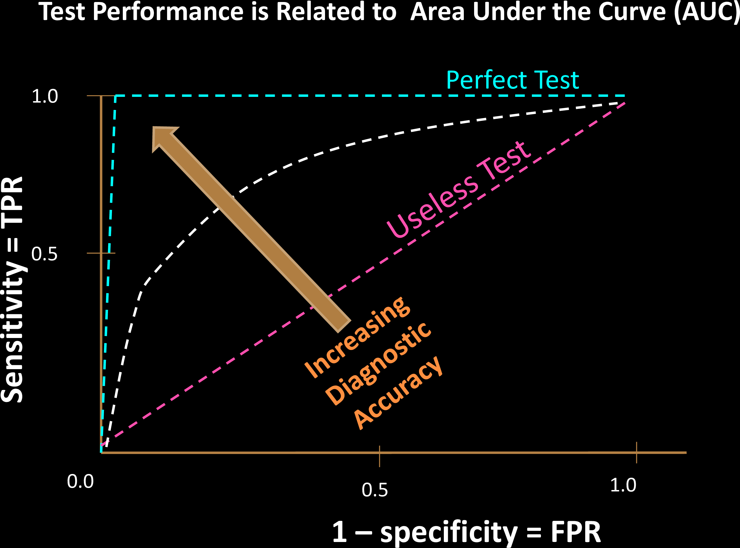
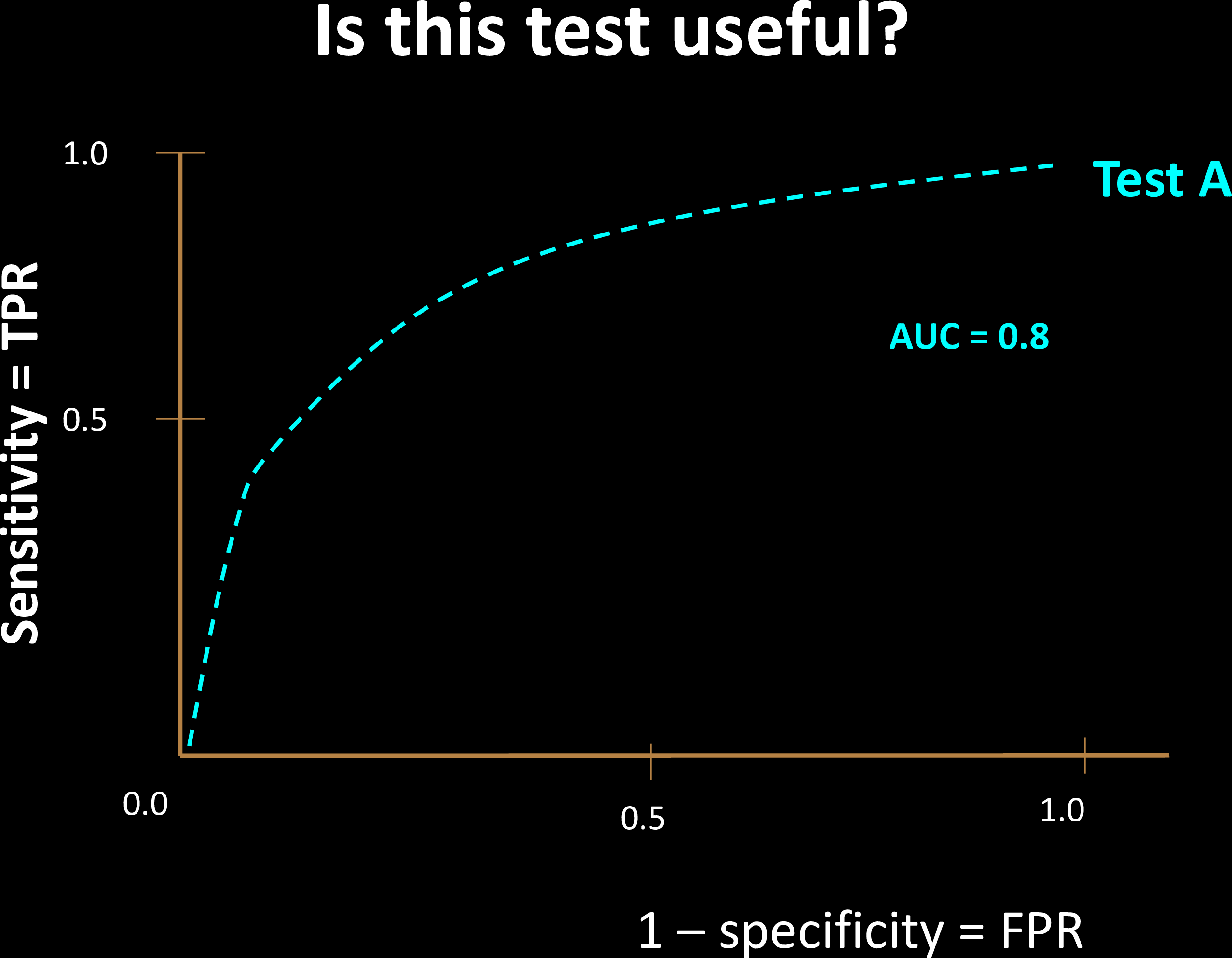
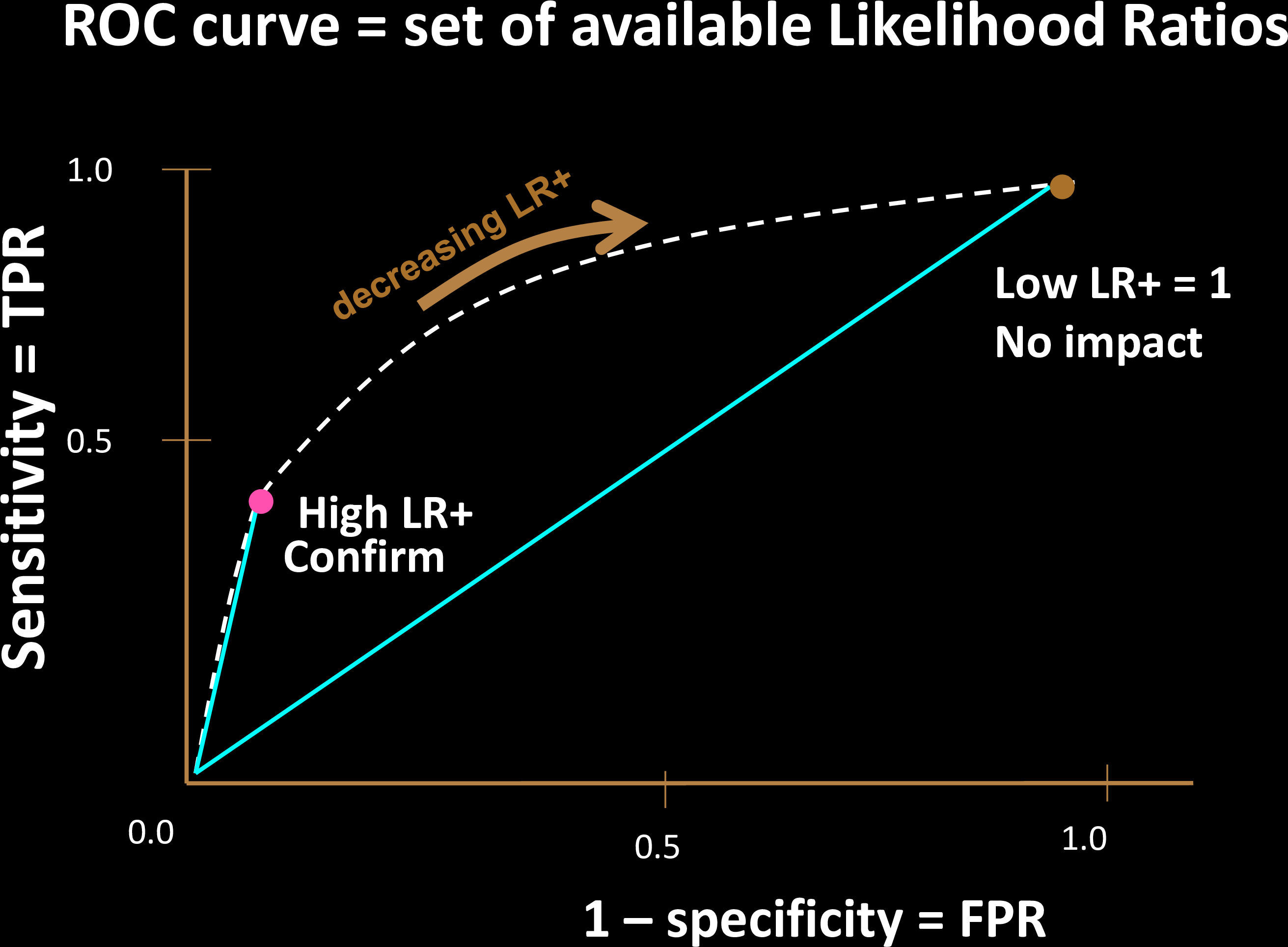
Comparing Tests
Comparing Tests
Comparing Tests
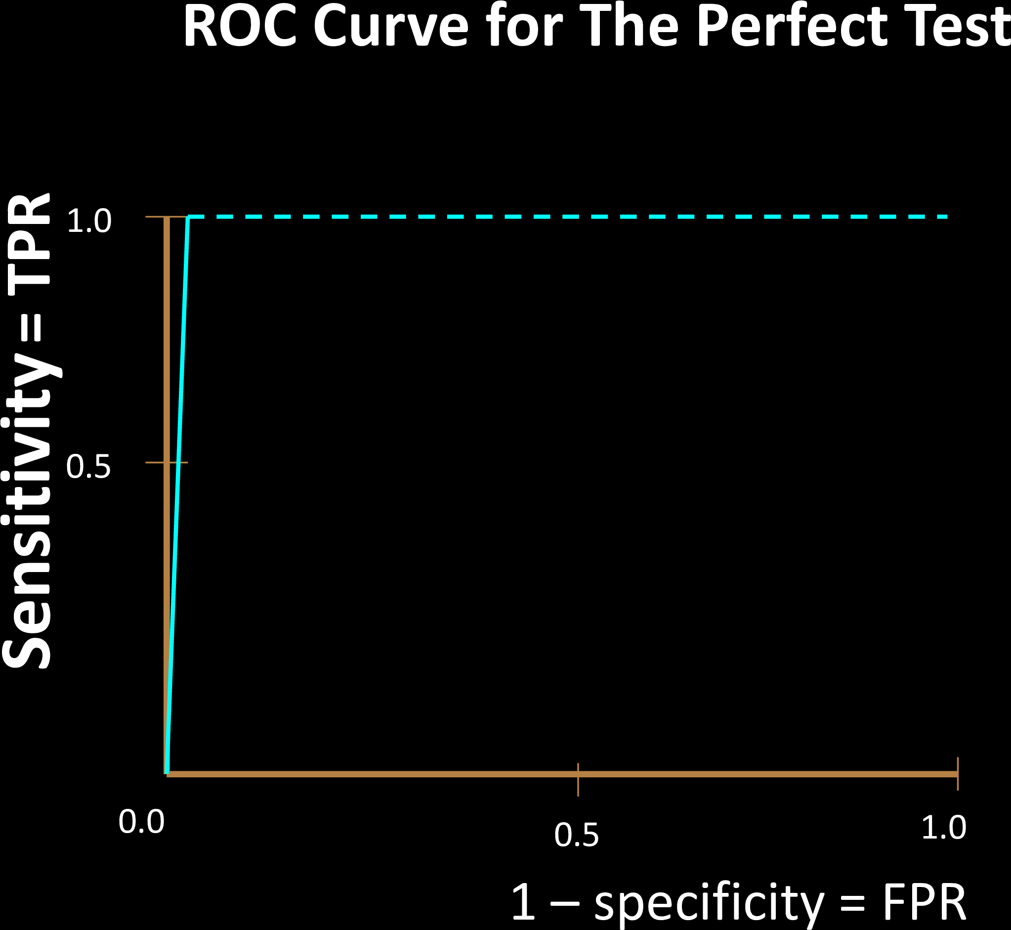
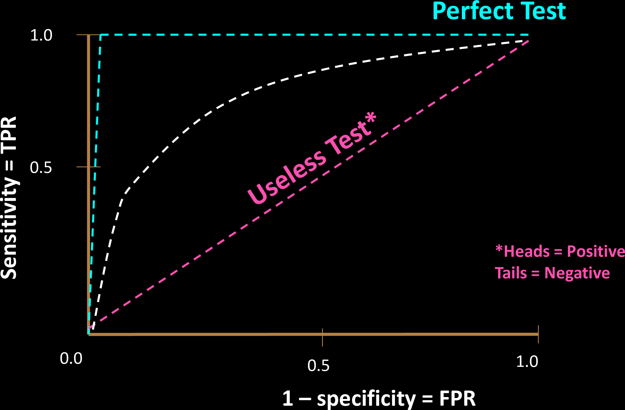
Why is a "diagonal ROC" useless?
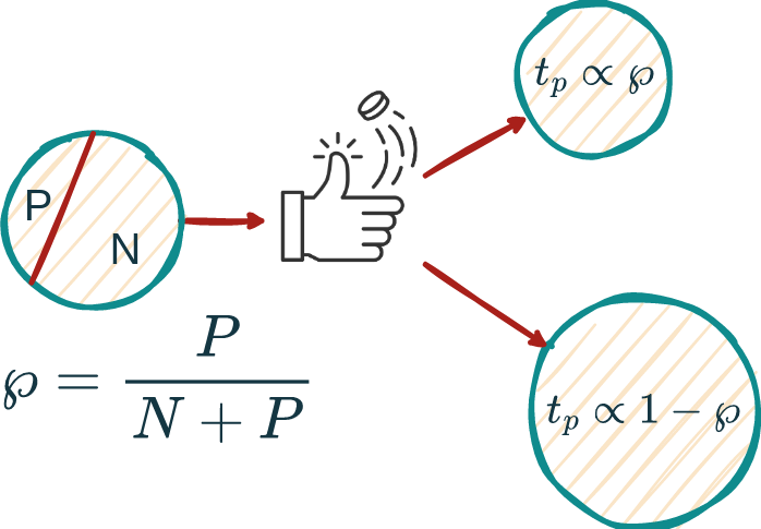
Let sensitivity be \(s\), specificity be \(c\), and prevalence P/(N+P) be \(\wp\).
Then:
Hence, s=c is NO BETTER than a coin toss!
Comparing Tests
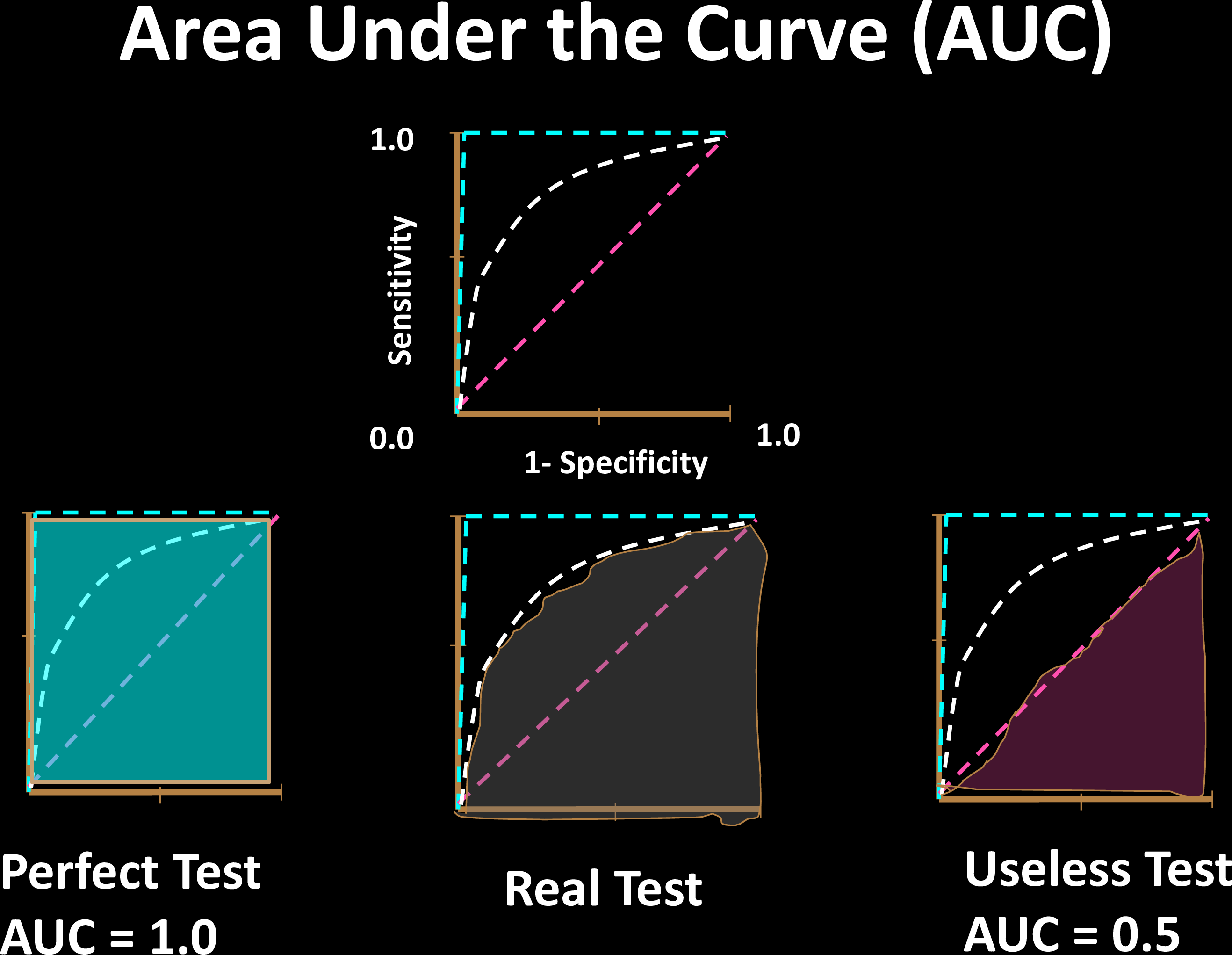
Comparing Tests

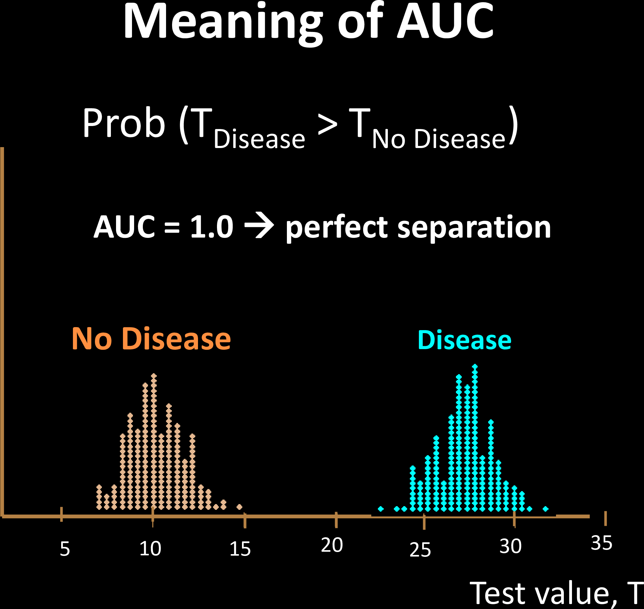
- AUC only considers ranks, not actual values
- Related to the Mann-
Whitney U Test - Shows why AUC is immune to class imbalence
For 2 random samples, AUC is the probability that the positive sample is ranked higher than the negative one

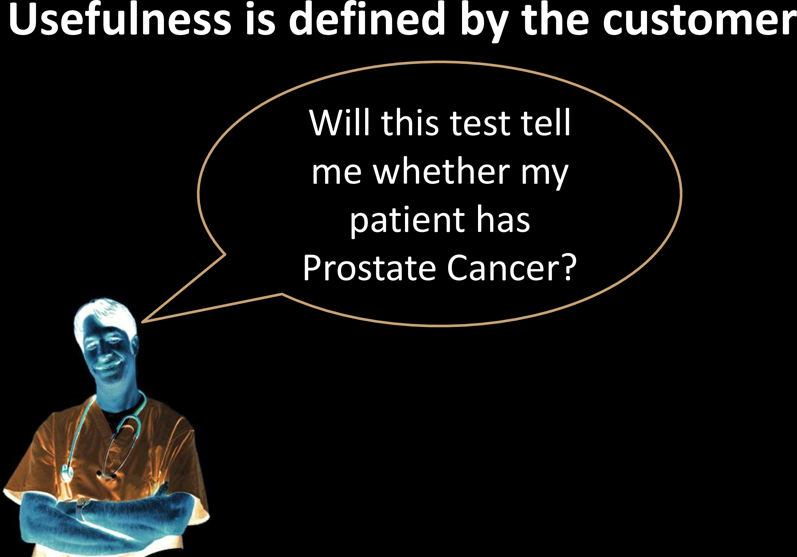


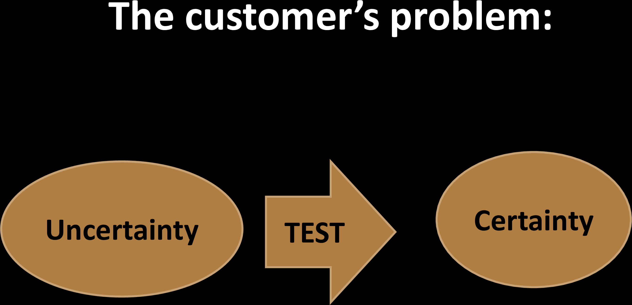
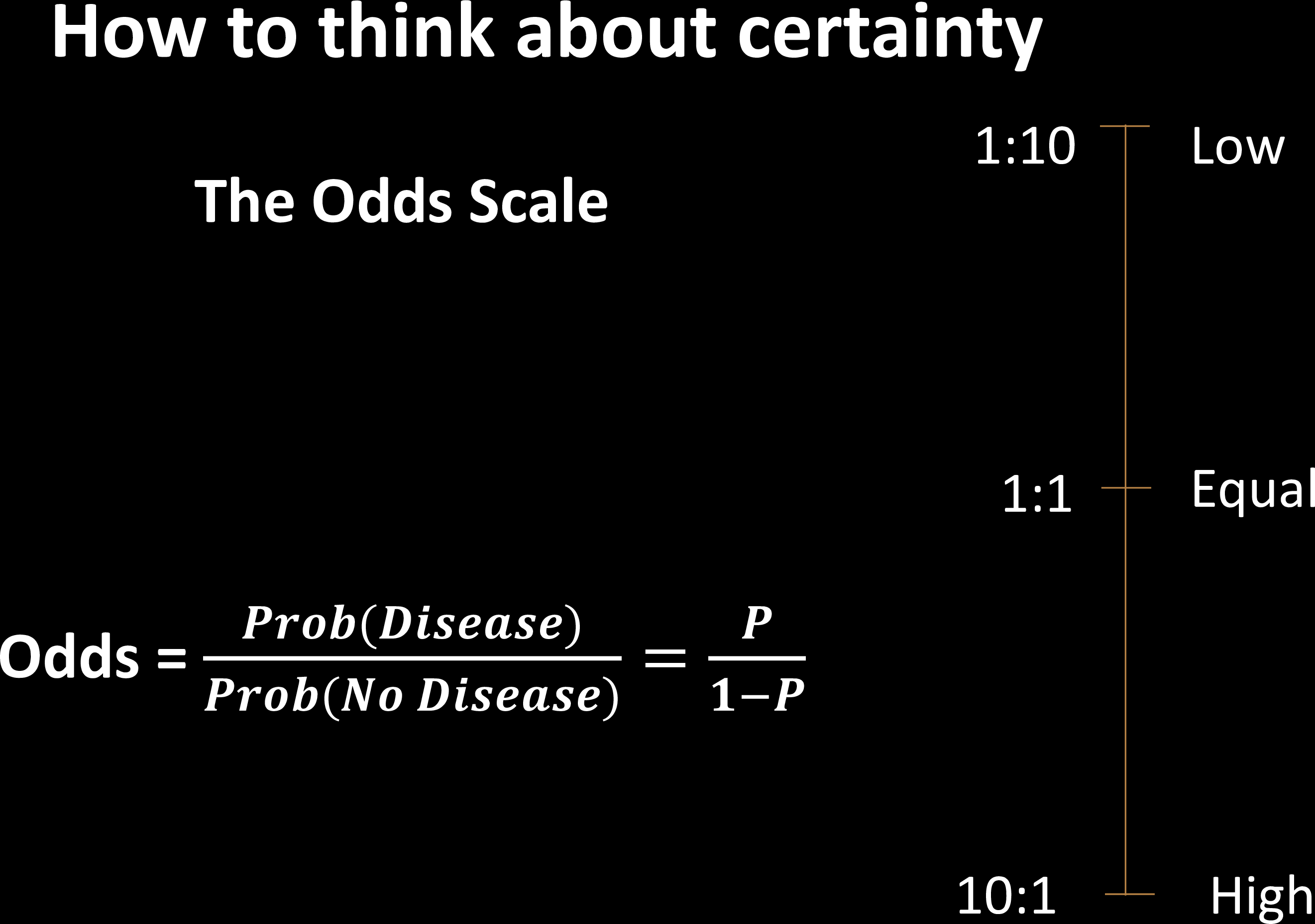
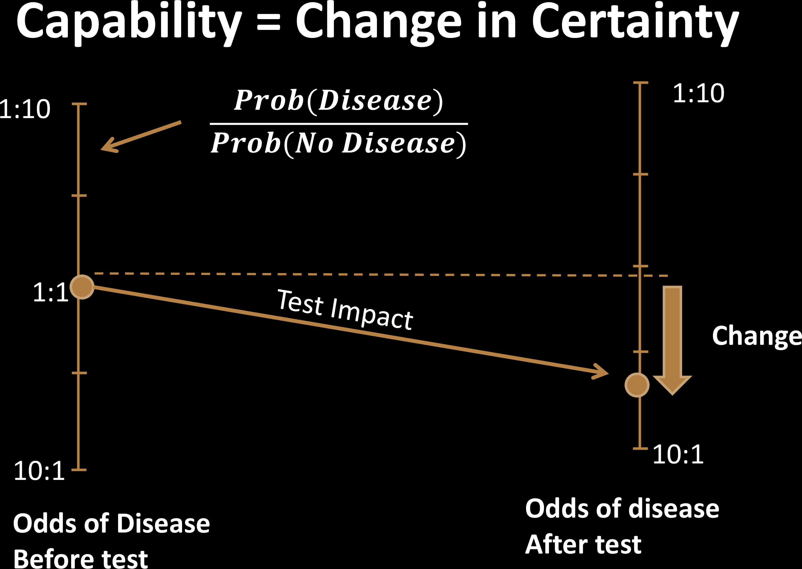
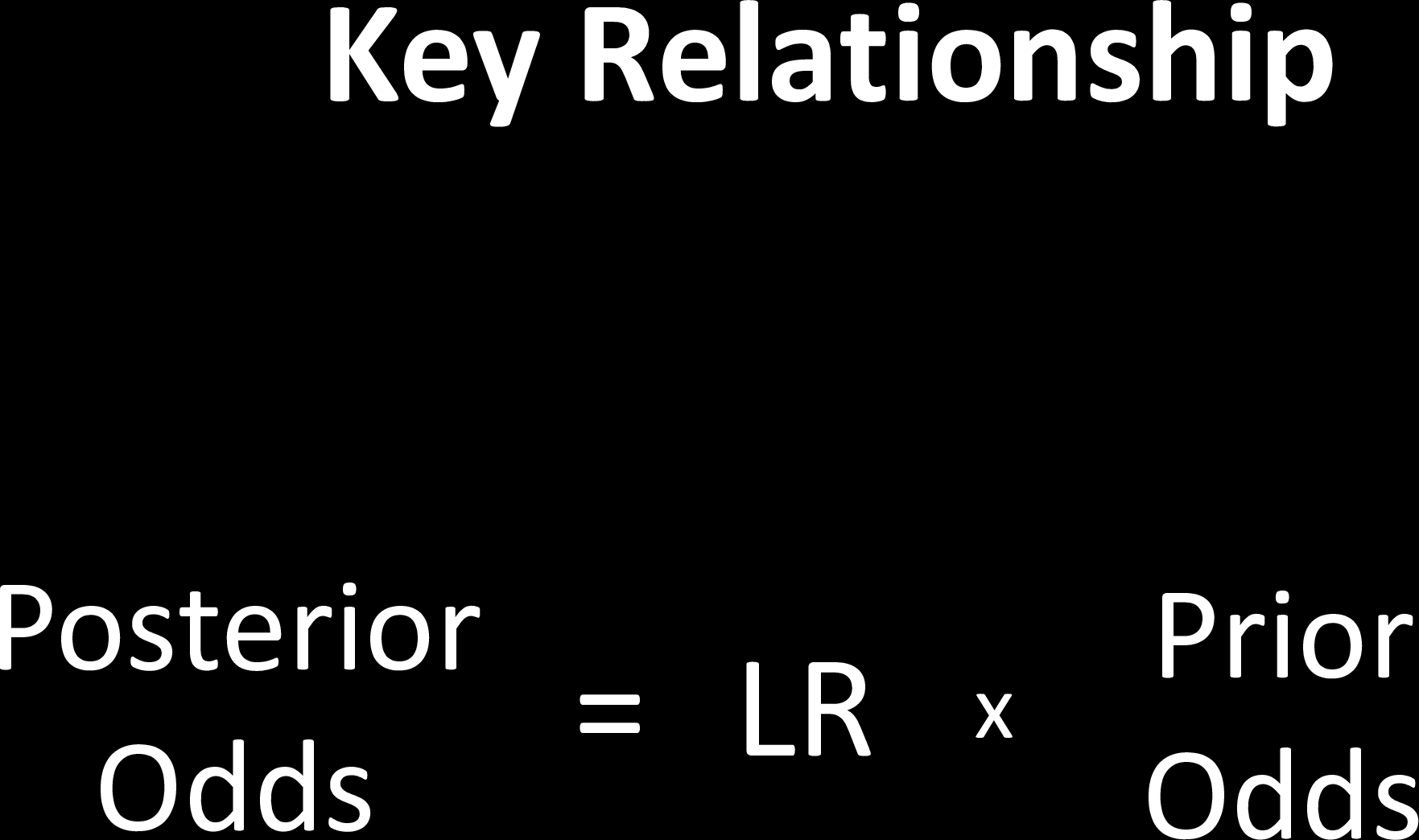
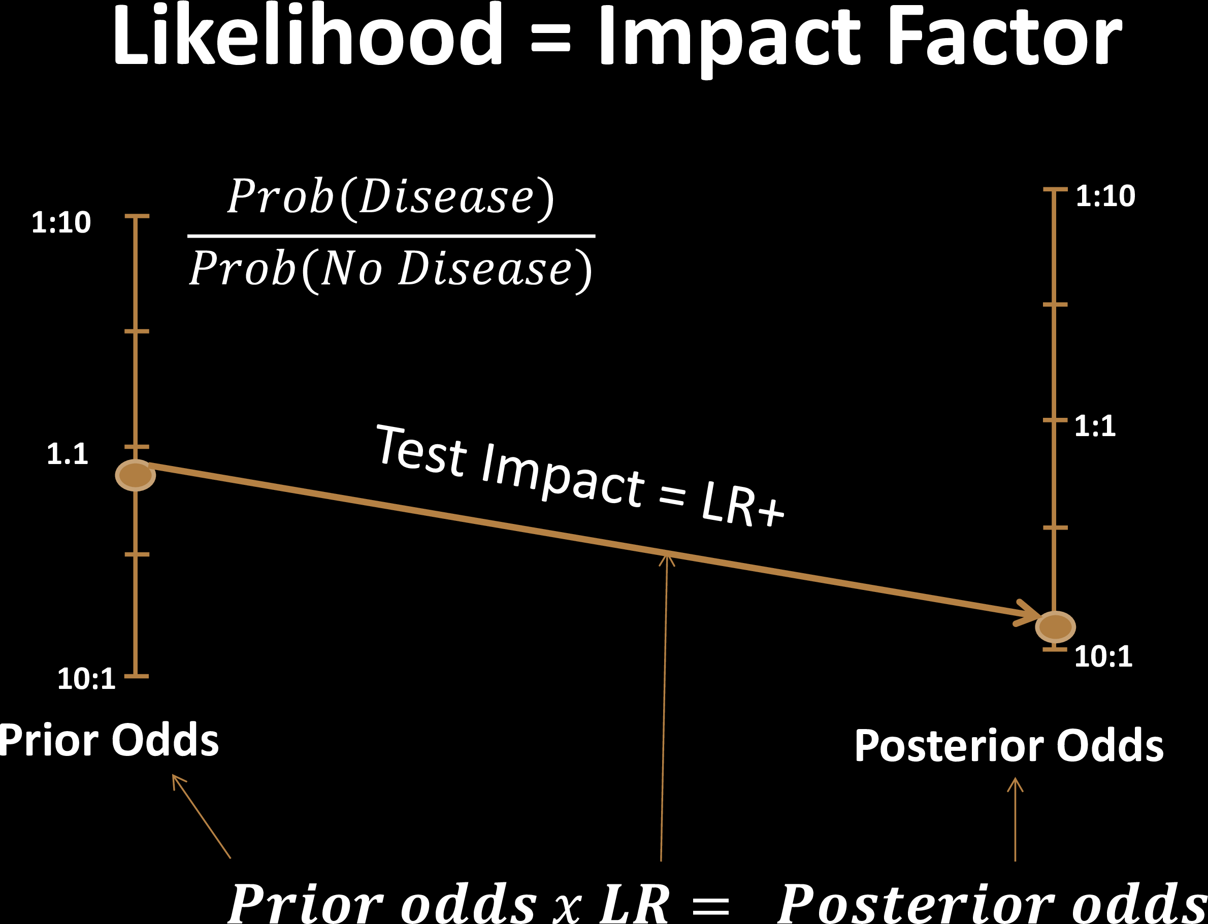
Tests are tools to reduce uncertainty
Test Effectiveness
Test Effectiveness
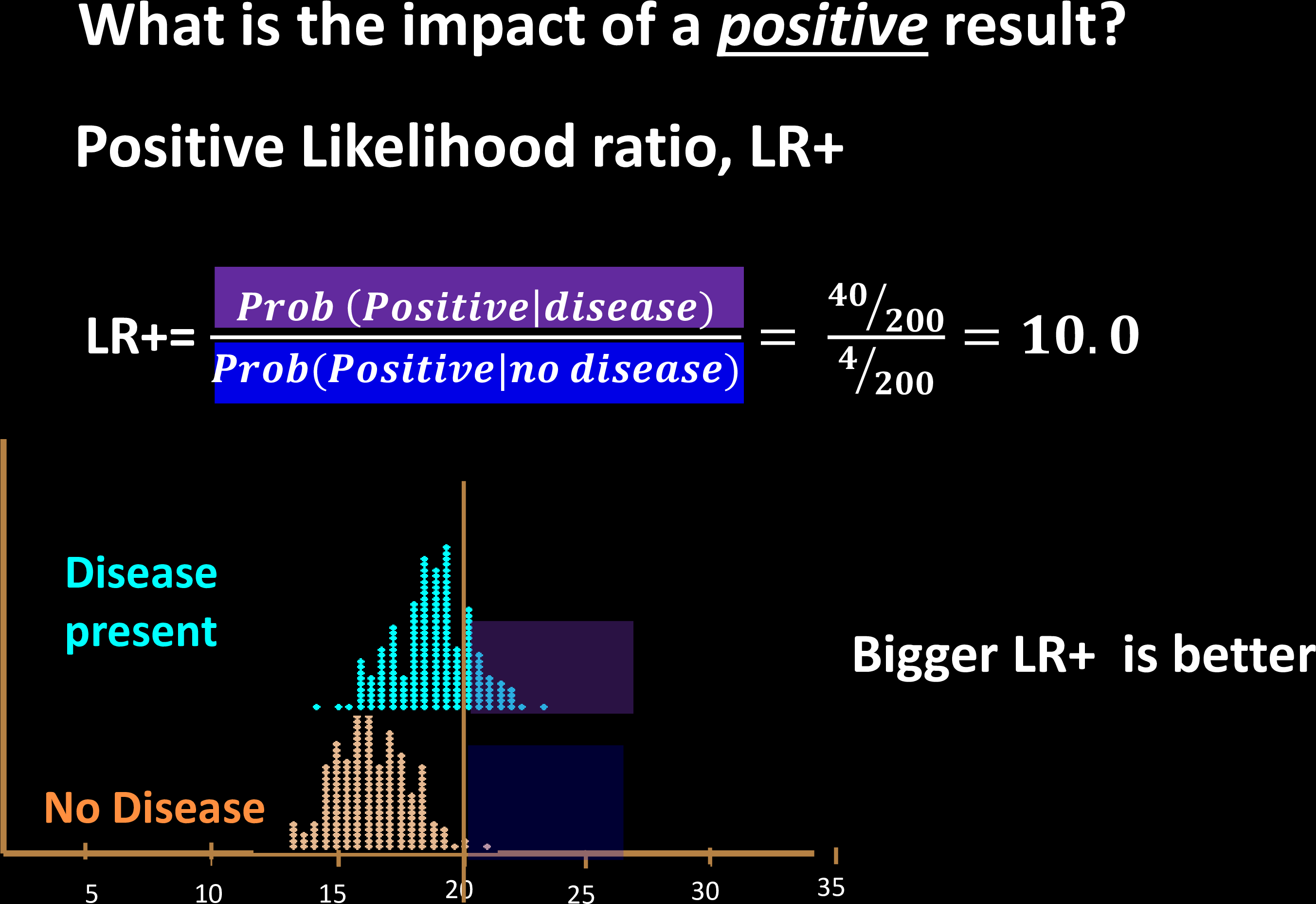
Test Effectiveness
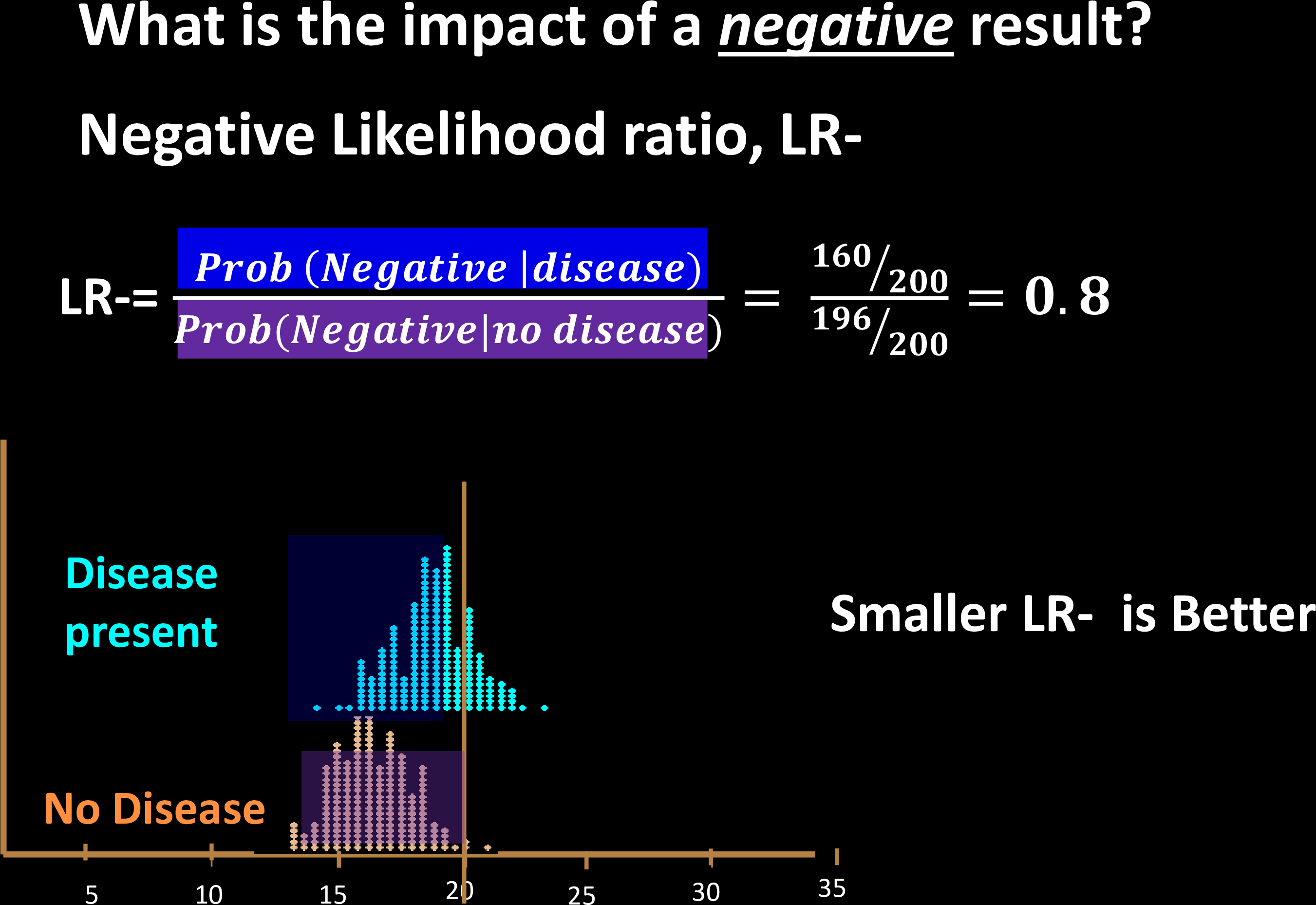
Test Effectiveness
Prove this using Bayes' Theorem
Test Effectiveness
$$t_p/f_p$$
$$\frac{\rho}{1-\rho}$$
Test Effectiveness
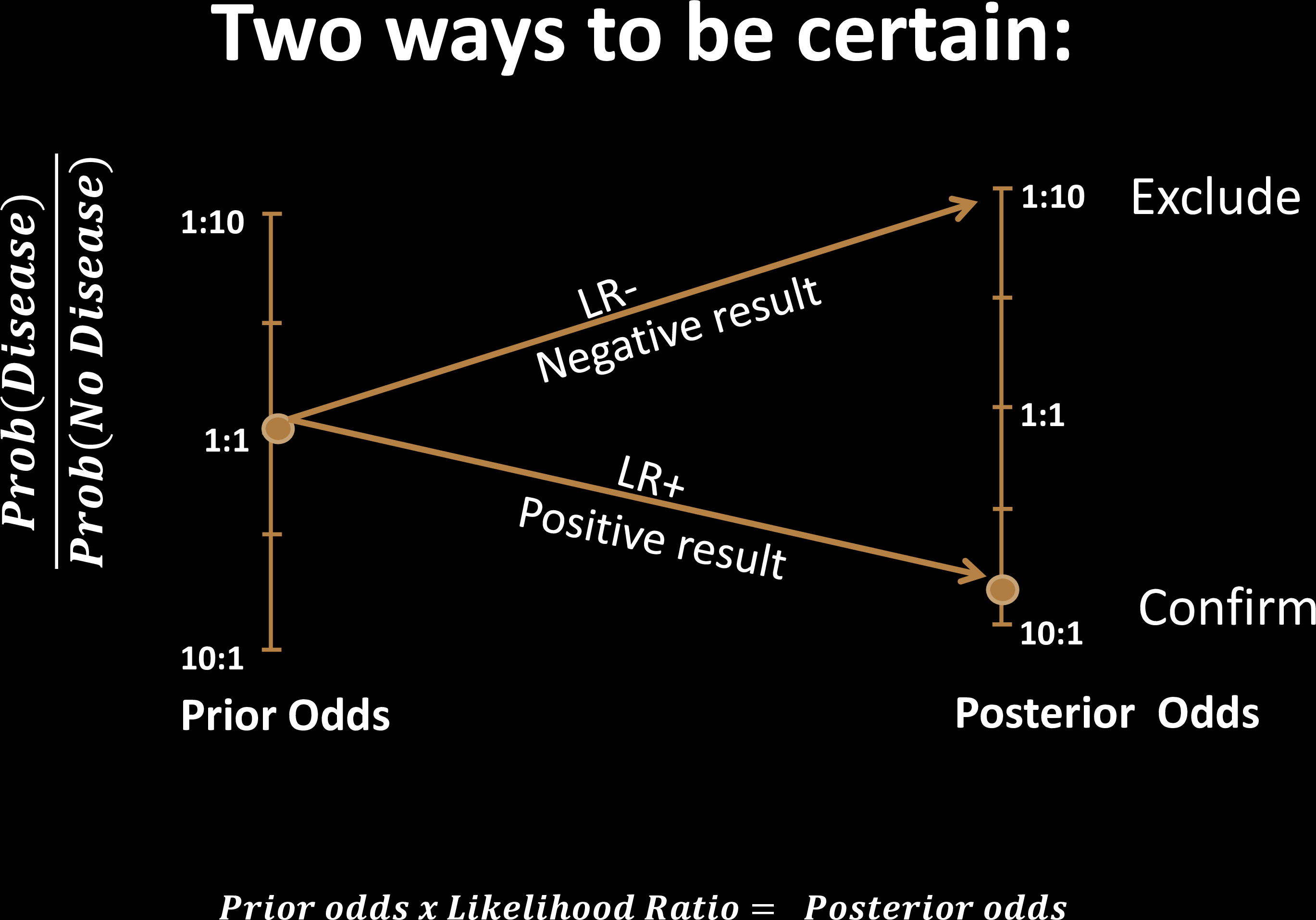
Test Effectiveness
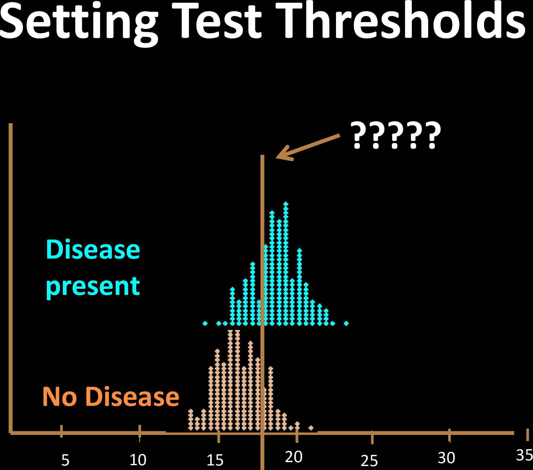
Choosing Thresholds
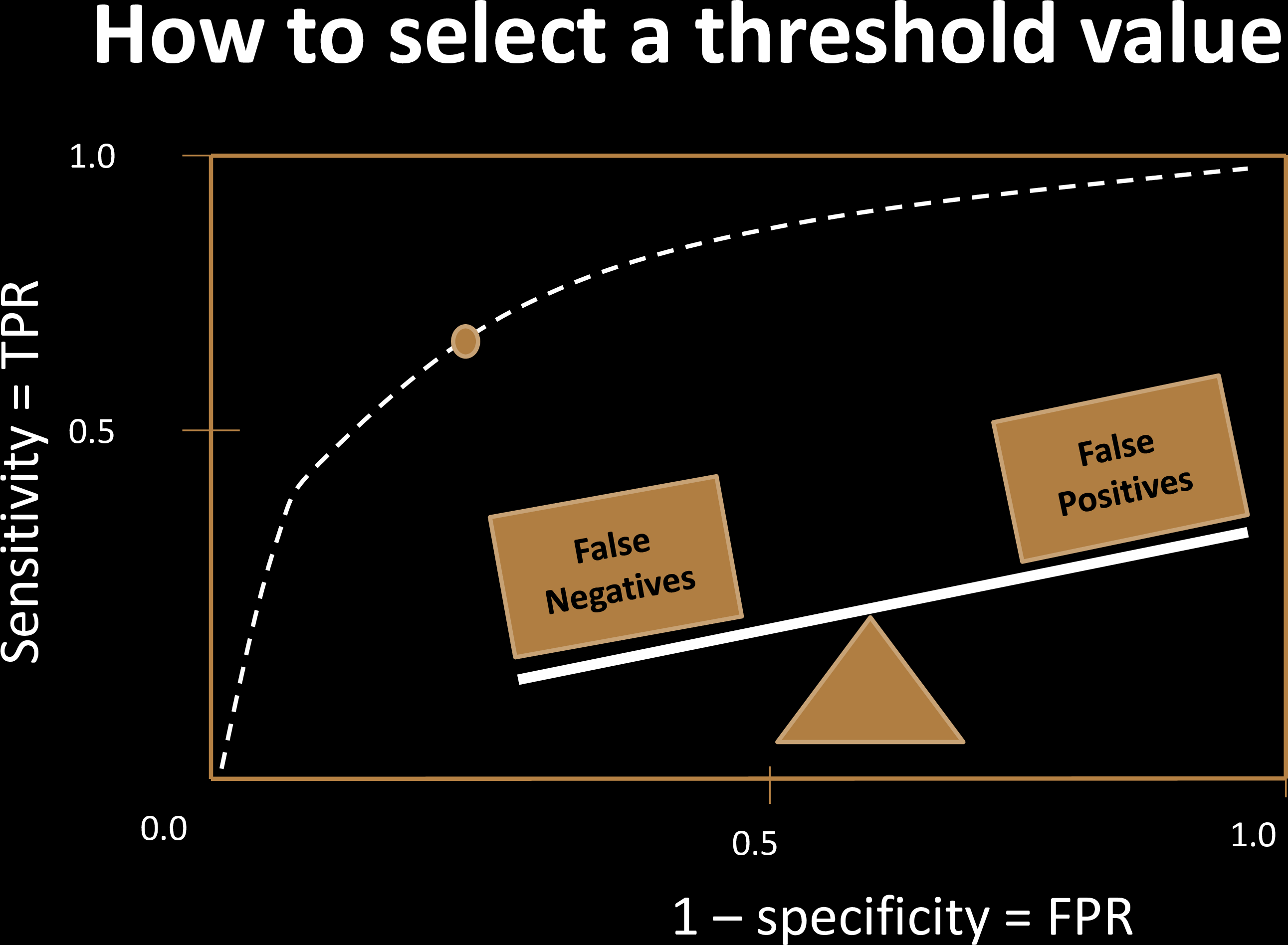
Balancing False Positives & False Negatives
| Cost | Positive | Negative |
|---|---|---|
| Test Positive | $0 | $x |
| Test Negative | $y | $0 |
Cost Optimization to choose operating point
Criminal Justice: $$C(f_n) = 0 $$
Healthcare (Covid test?)
$$C(f_p) = 0 $$
naive dichotomy
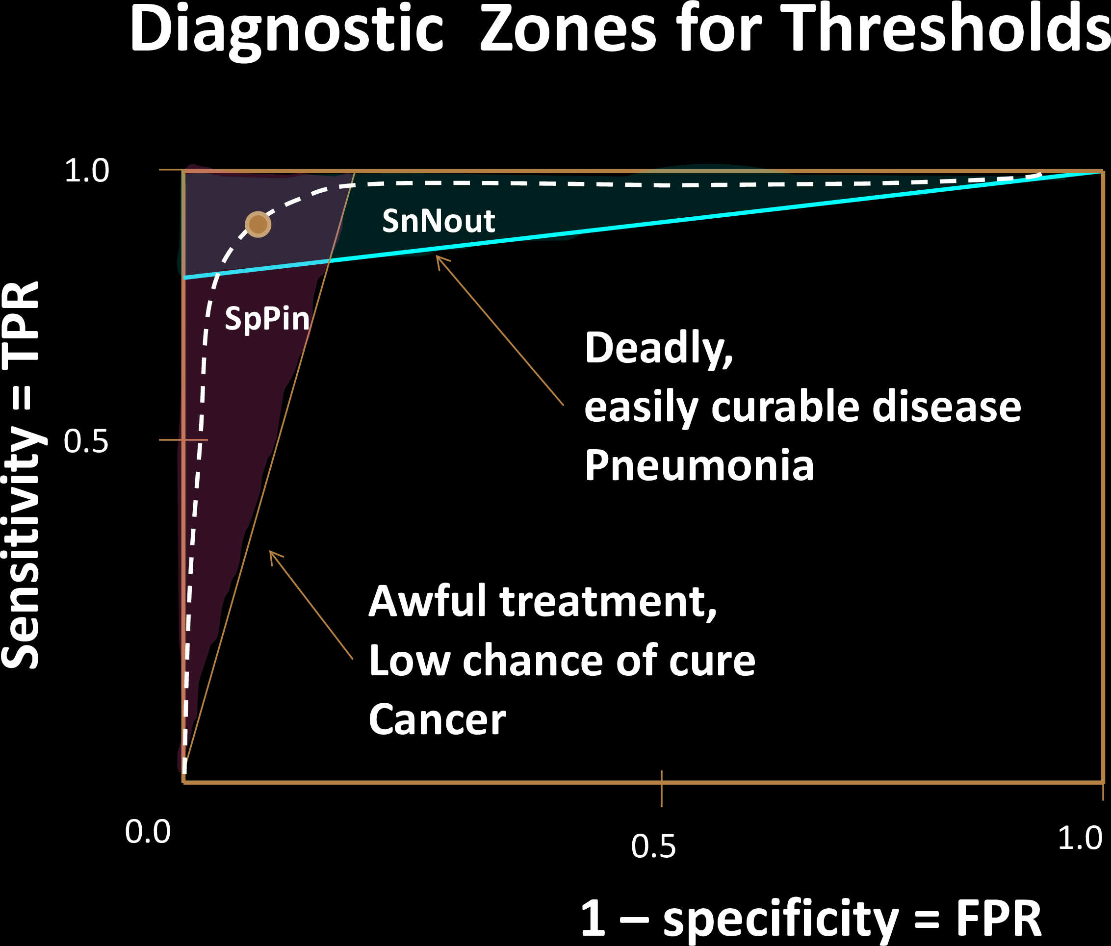
Choosing Thresholds
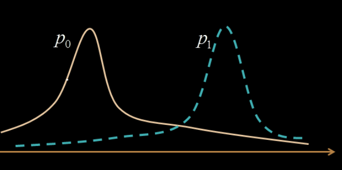
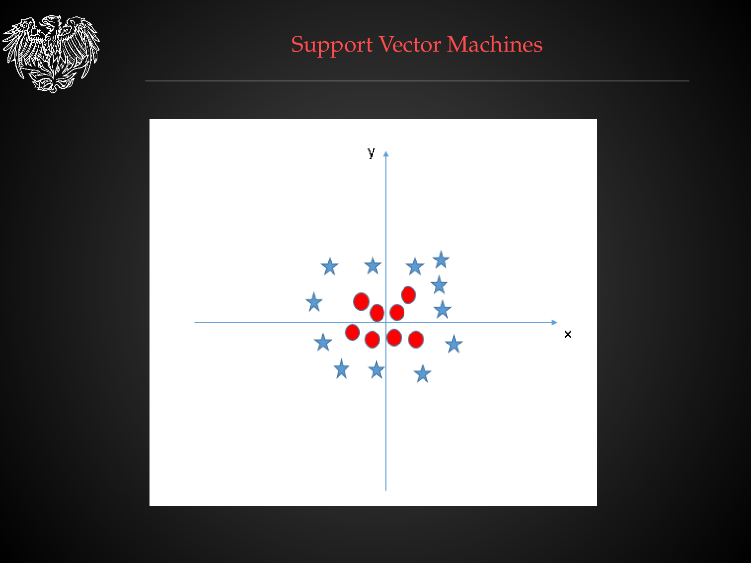
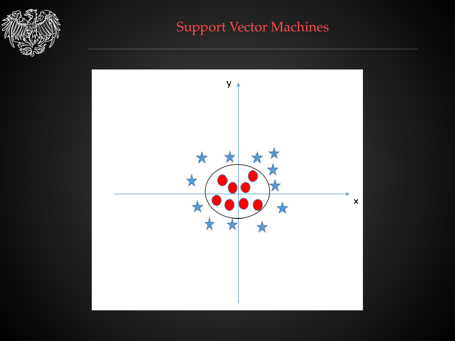
Overlapping features are harder to classify
How do we formalize these trade-offs?

What happens if we test again?
0.045
0.045
1-0.045
0.69
But confirmatory tests might not be always feasible
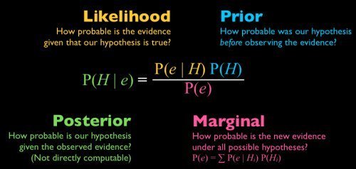
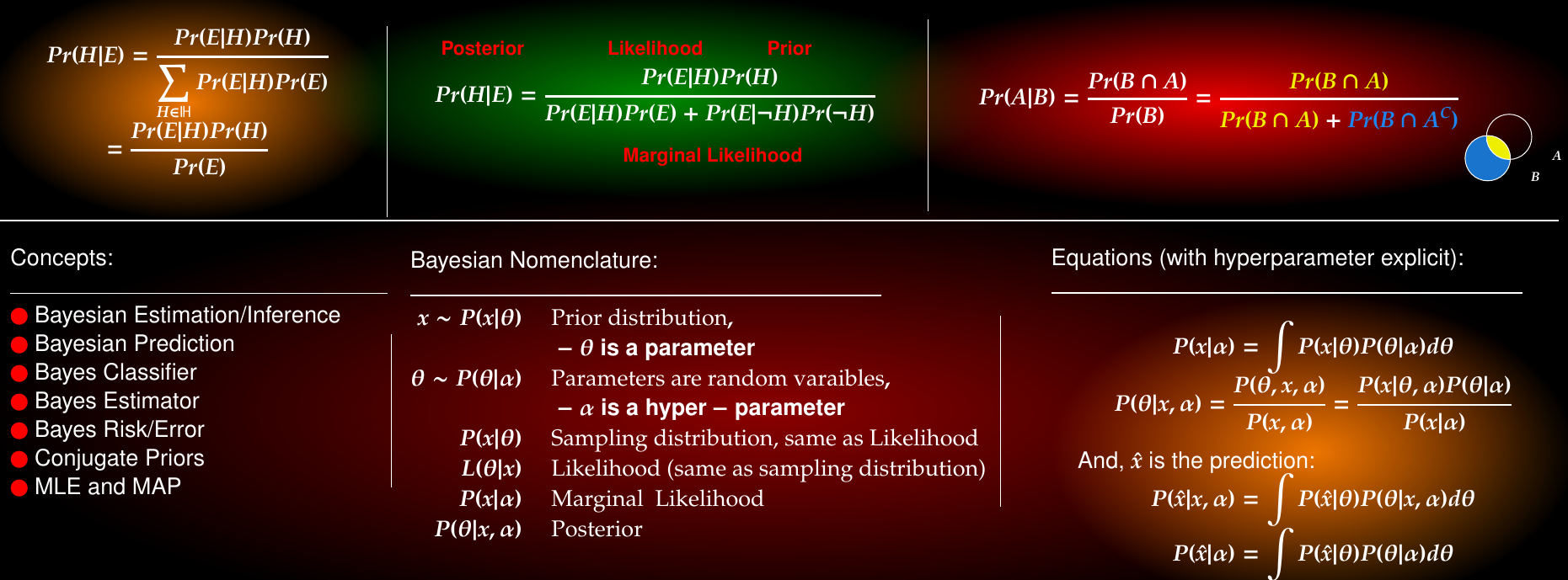
Summary of Bayesian Inference
(H)
Bayes' Error
Classification & Decision Theory
Classification & Decision Theory
Classification & Decision Theory
Bayes Risk
Risk of a classifier:
Mathematical definition of classifier:
search over all possible classifiers
A classifier achieving the Bayes risk is a Bayes Optimal Classifier
Classification & Decision Theory
Bayes Risk
A classifier achieving the Bayes risk is a Bayes Optimal Classifier
Bayesian Decision Theory
Minimizing the 0, 1-loss is equivalent to minimizing the overall misclassification rate. 0, 1-loss is an example of a symmetric loss function: all errors are penalized equally. In certain applications, asymmetric loss functions are more appropriate.
Recall cost of false negatives vs that of false positives
The expected 0, 1-loss is precisely the probability of making a mistake
Defining Bayes Optimal Classifier in terms of the Loss function
Bayesian Decision Theory
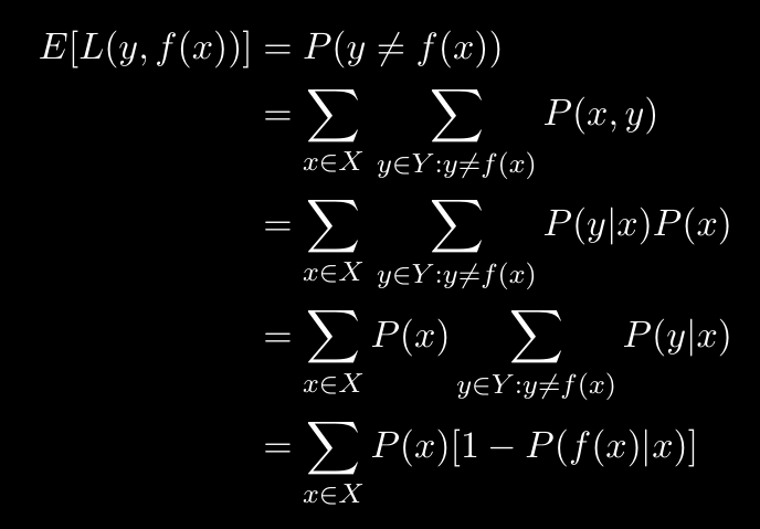
Bayes Optimal Classifier
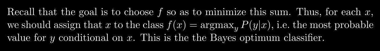
The above derivation is of course for only 0-1 Loss
But this is true in general
Bayes Risk
Bayes Risk

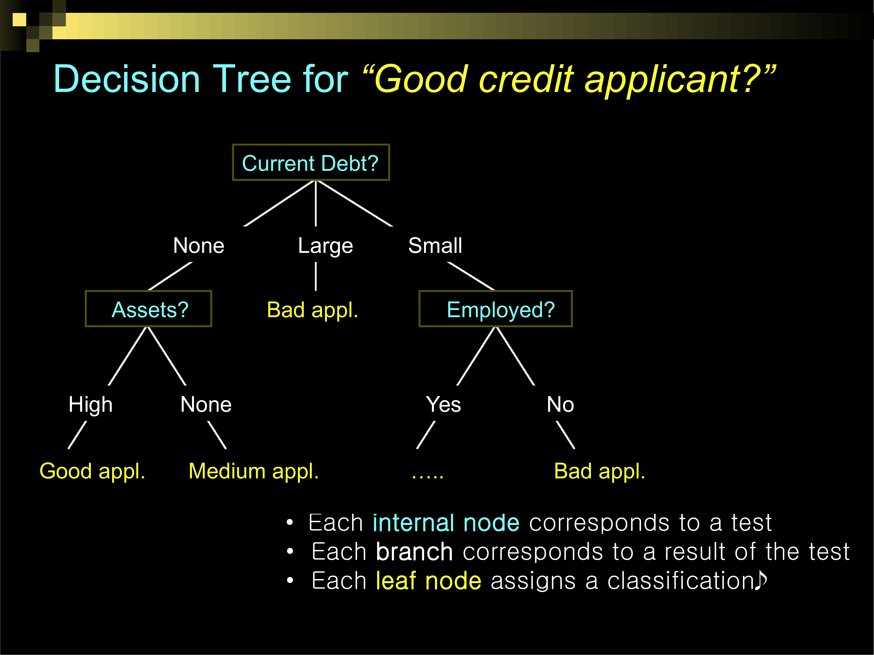
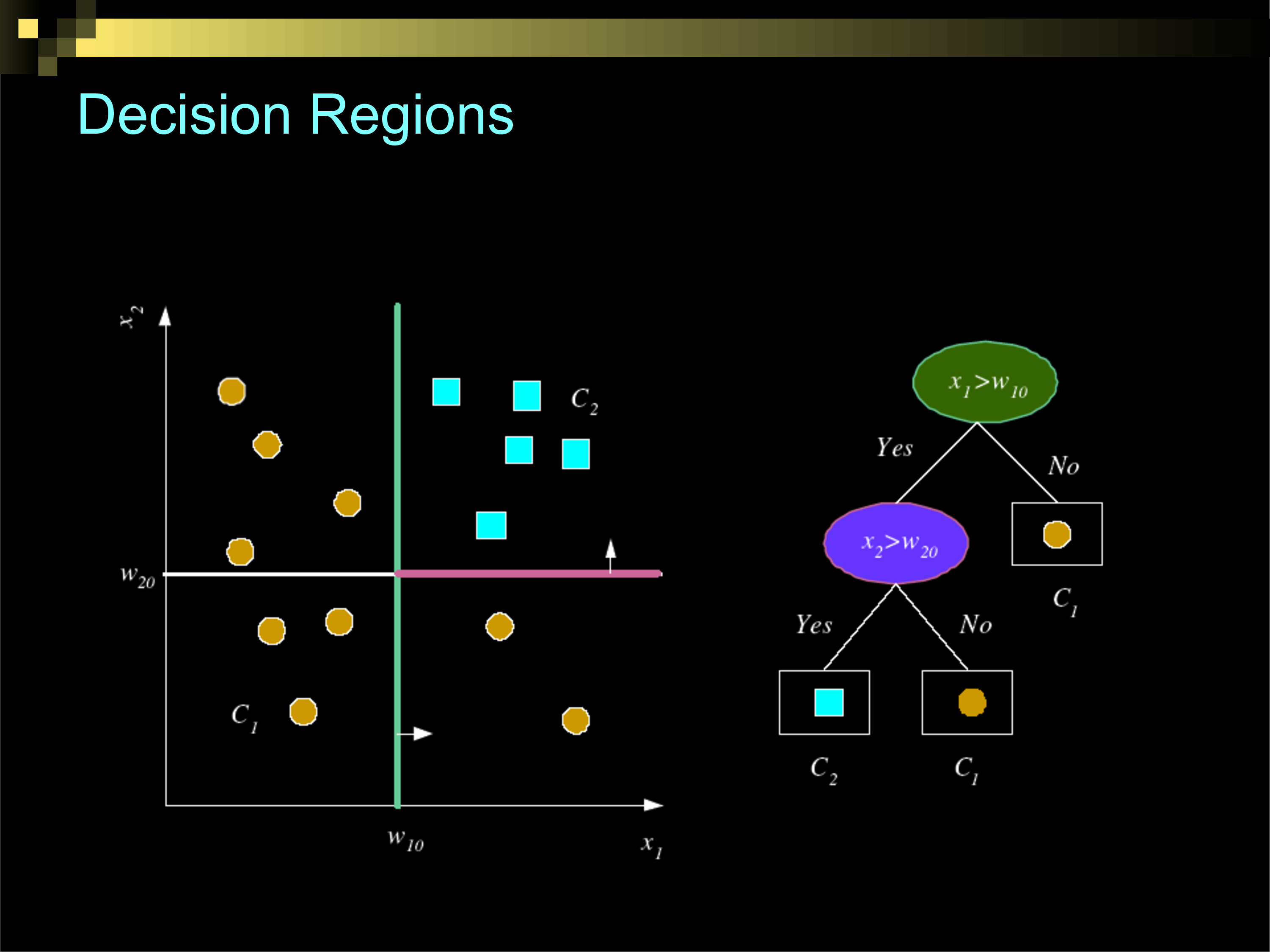
Decision Trees
Books
-
Antonio Criminisi, Jamie Shotton (2013)
- [Decision Forests for Computer Vision and Medical Image Analysis] (http://link.springer.com/book/10.1007%2F978-1-4471-4929-3)
-
Trevor Hastie, Robert Tibshirani, Jerome Friedman (2008)
- [The Elements of Statistical Learning, (Chapter 10, 15, and 16)] (http://web.stanford.edu/~hastie/local.ftp/Springer/OLD/ESLII_print4.pdf)
- Luc Devroye, Laszlo Gyorfi, Gabor Lugosi (1996)
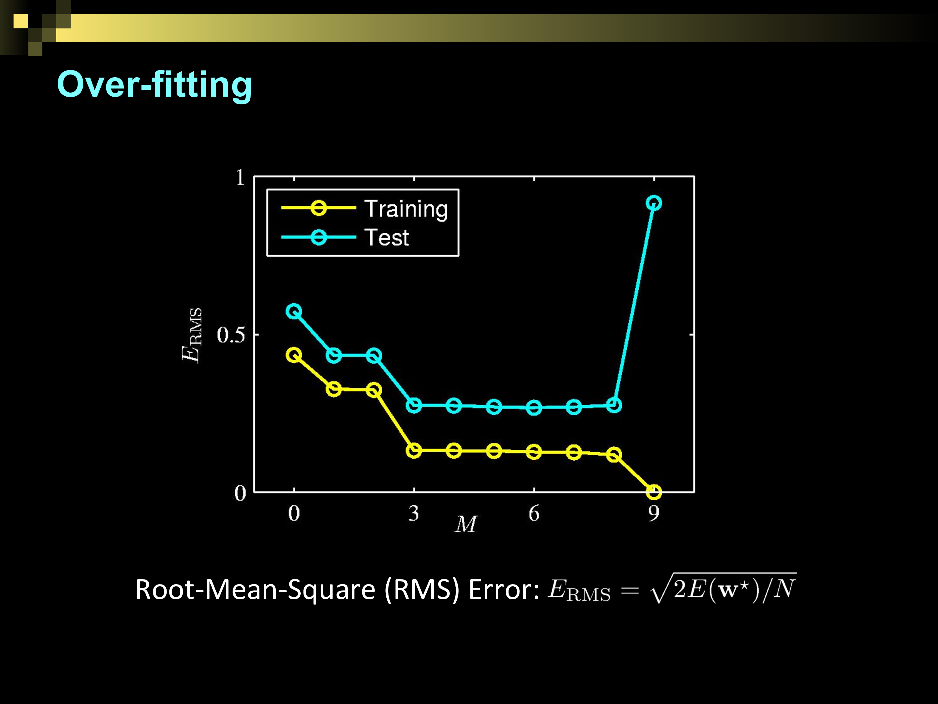
Overfitting
How do we make decision trees better?
Reduce "bias"
Reduce "variance"
Cannot reduce "irreducible error"
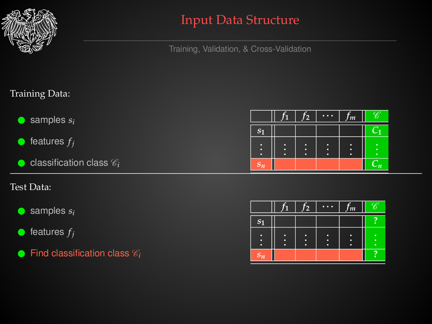
THE TABULAR DATA FORMAT
Summing Up The ML Problem

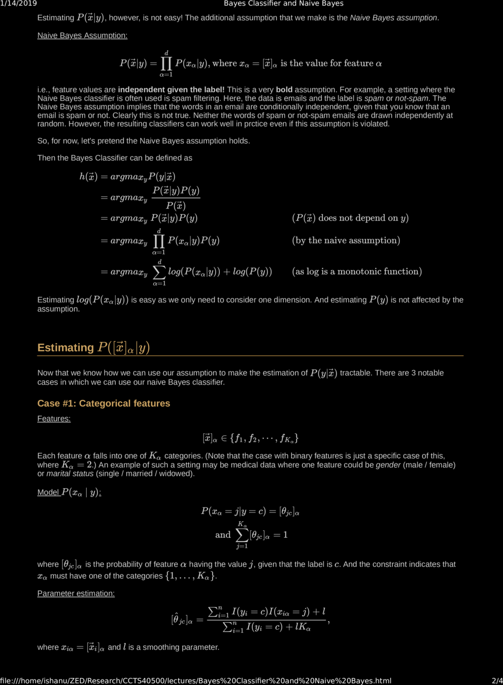
Naive Bayes Assumption

Vox Populi Vox Dei
OK, Back to Making Decision Trees Better.....
Vox Populi Vox Dei
OK, Back to Making Decision Trees Better.....
Bias Variance, Reducible & Irreducible Error
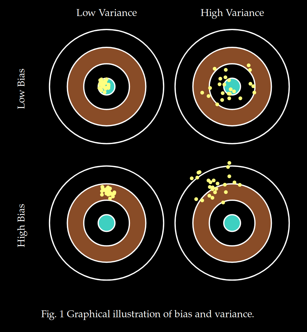
Bias Variance, Reducible & Irreducible Error
Bias Variance, Reducible & Irreducible Error
Expected Test Error:
bias
variance
irreducible error

from sklearn.model_selection import train_test_split
from sklearn import metrics
from sklearn.tree import DecisionTreeClassifier
from sklearn.ensemble import BaggingClassifier

clf_ = DecisionTreeClassifier(max_depth=4, class_weight='balanced')
clf = BaggingClassifier(base_estimator=clf_,n_estimators=10,oob_score=True)
X_train, X_test, y_train, y_test = train_test_split(X, y, test_size=0.2)
clf.fit(X_train,y_train)
clf.predict(X_test,y_test)
Feature Importance for Bagging Classifier
import numpy as np
from sklearn.ensemble import BaggingClassifier
from sklearn.tree import DecisionTreeClassifier
from sklearn.datasets import load_iris

X, y = load_iris(return_X_y=True)
clf = BaggingClassifier(DecisionTreeClassifier())
clf.fit(X, y)

feature_importances = np.mean([
    tree.feature_importances_ for tree in clf.estimators_
], axis=0)
Average over the feature importance of base models
Median might be better
- Results no longer easily interpretable
- One can no longer trace the "logic" of an output through a series of decisions based on predictor values
Problem with Ensemble Methods
Instead of one "rule", it is a distribution over rules, or a linear combination of rules
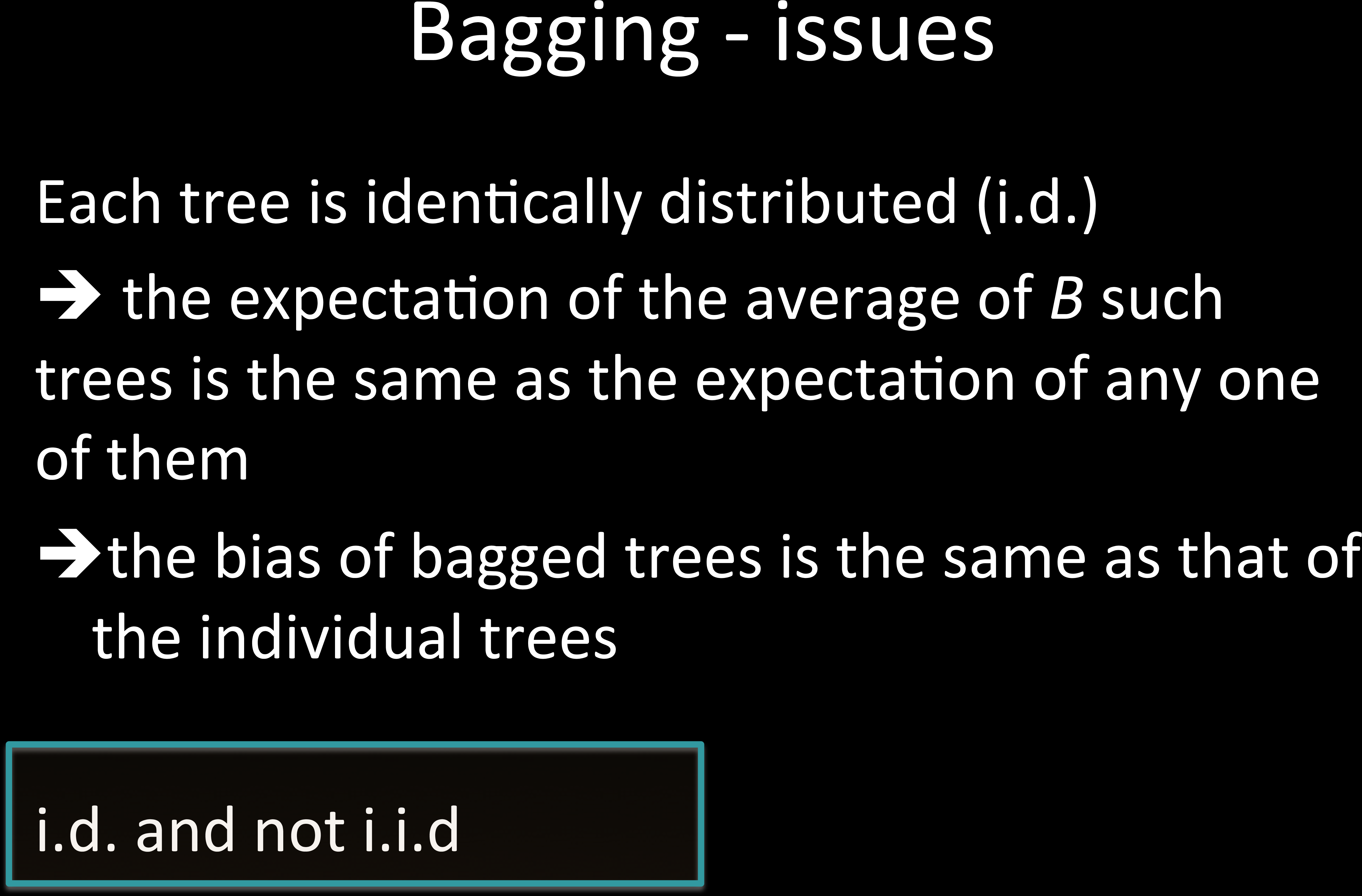
What happens when there is one strongly predicting feature?
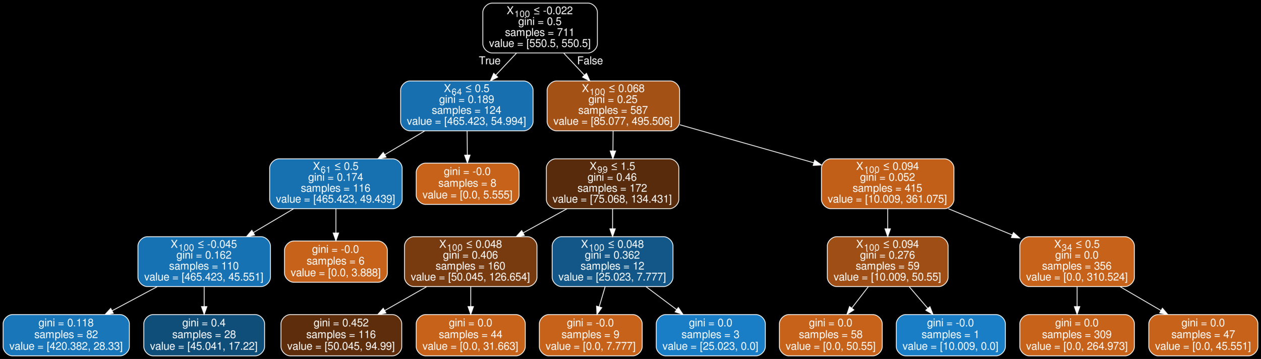
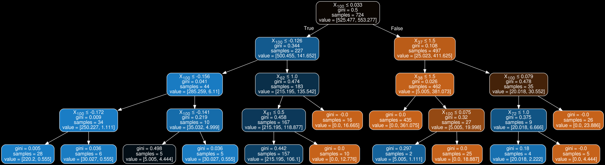
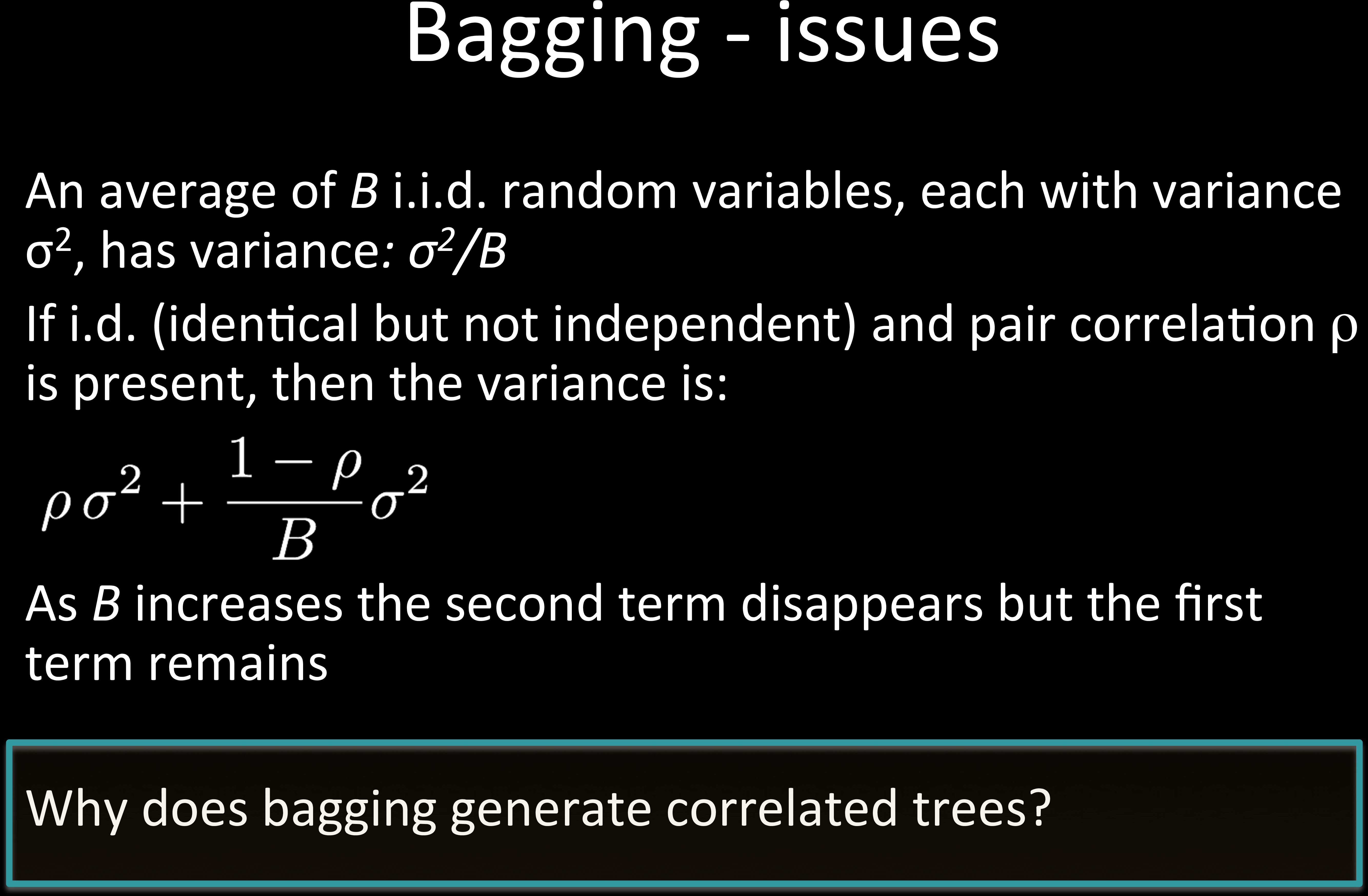
How do we avoid this?
We can penalize the number of times a feature is used at a certain depth
We can penalize the number of times a feature can be used
We will only allow some features chosen by some meta analysis
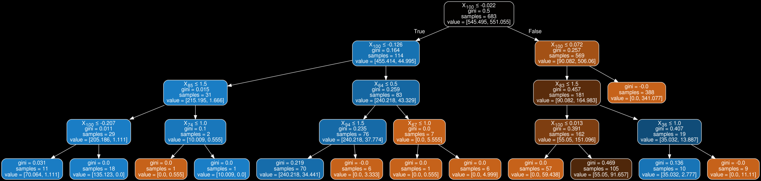
No! Same Bias
No! Same Bias
No! Same Bias
features
samples
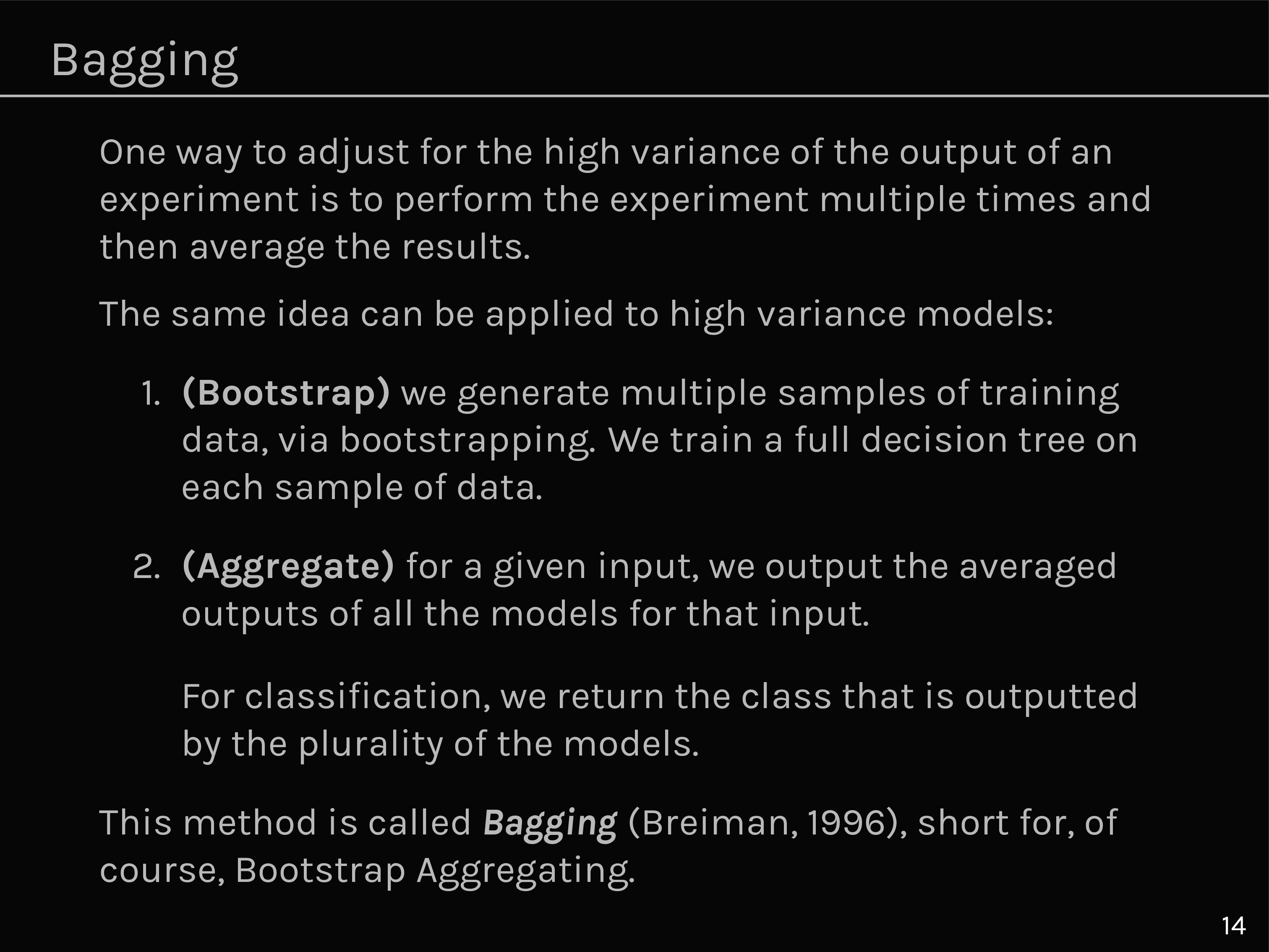
Bagging
features
samples
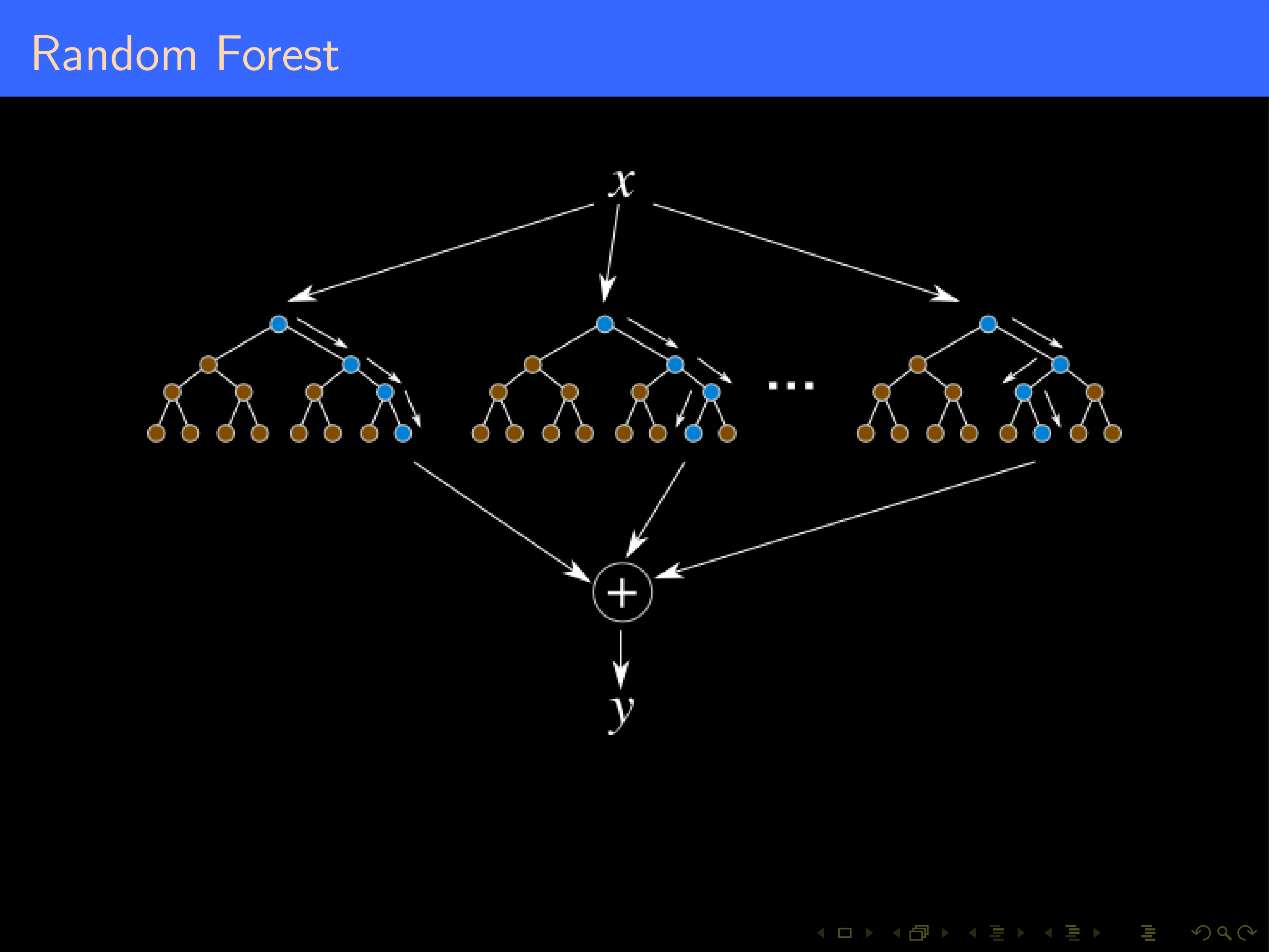
Random Forest

from sklearn.ensemble import RandomForestClassifier
clf = RandomForestClassifier(max_depth=None, class_weight='balanced',n_estimators=300)
y_pred = clf.fit(X_train, y_train).predict(X_test)
HW 1
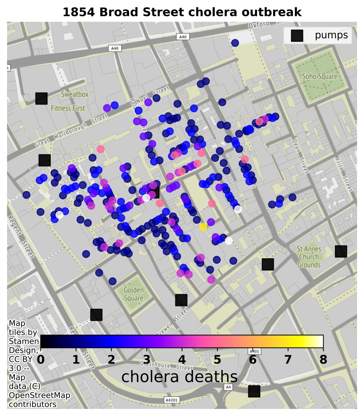
Theodore H. Tulchinsky, "John Snow, Cholera, the Broad Street Pump; Waterborne Diseases Then and Now", Case Studies in Public Health. 2018 : 77–99 https://www.ncbi.nlm.nih.gov/pmc/articles/PMC7150208/
- Cholera was a major global scourge in the 19th century, with frequent large-scale epidemics in European cities primarily originating in the Indian subcontinent.
- John Snow conducted pioneering investigations on cholera epidemics in England and particularly in London in 1854 i
- He demonstrated that contaminated water was the key source of the epidemics.
- His thorough investigation of an epidemic in the Soho district of London led to his conclusion that contaminated water from the Broad Street pump was the source of the disease and, consequently, the removal of the handle led to cessation of the epidemic.


Can you retrace J. Snow's argument?
The prevailing Miasma Theory was that cholera was caused by airborne transmission of poisonous vapors from foul smells due to poor sanitation. At the same time, the competing Germ Theory that inspired Snow was still an unproven minority opinion in medical circles.
1854 London
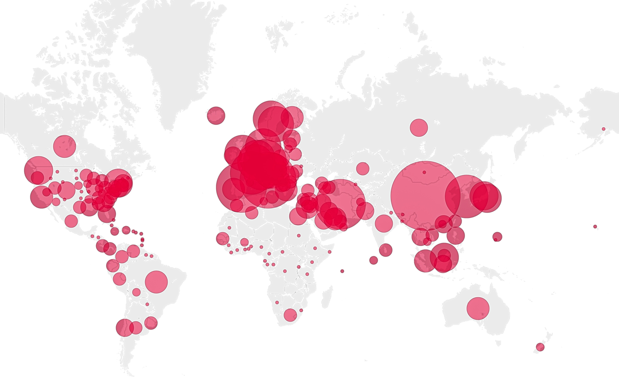
HW 2: Epidemiology of COVI-19 in US
# Question 1
+ Train a decision-tree to predict which counties experience a >5% change in daily count
+ Train a decision-tree to predict which counties experience a >5% change in weekly count
# Question 2
+ Redo Question 1 using a Bagging classifier. Try to optimize the number of estimators, and depth of tree in each estimator

ishanu_ch@uky.edu