


Content ITV PRO
This is Itvedant Content department
Learning Outcome
5
Evaluate and visualize a seasonal forecast
4
Use auto_arima to automatically find optimal seasonal parameters
3
Implement the SARIMAX algorithm using statsmodels
2
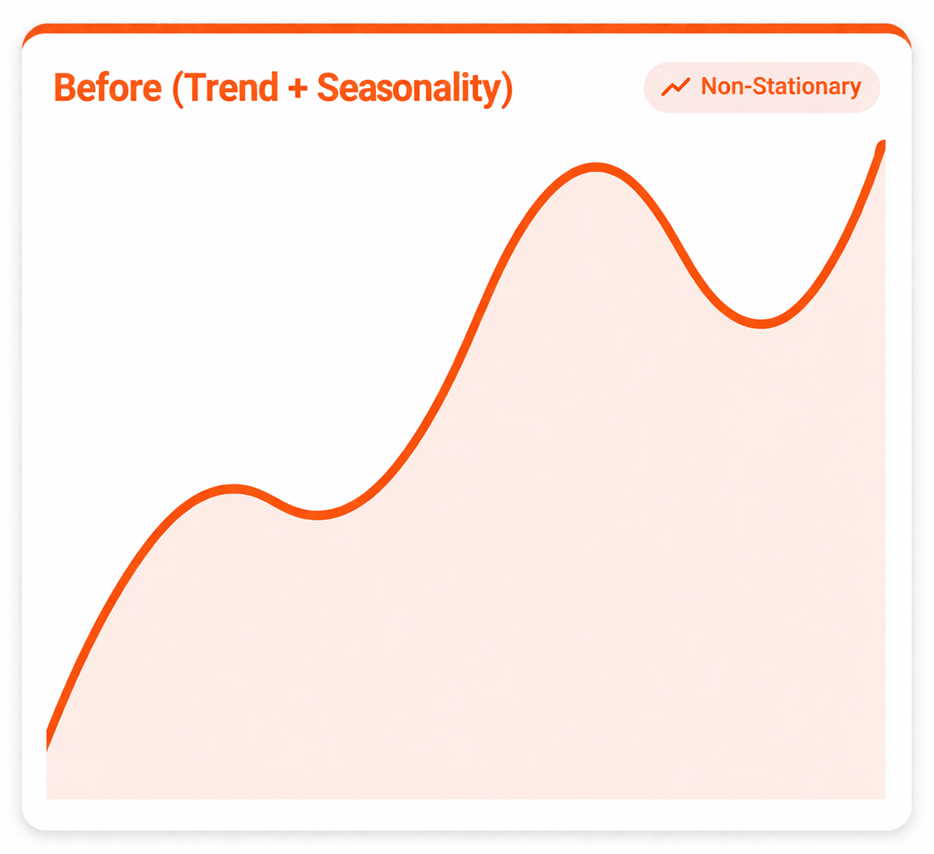
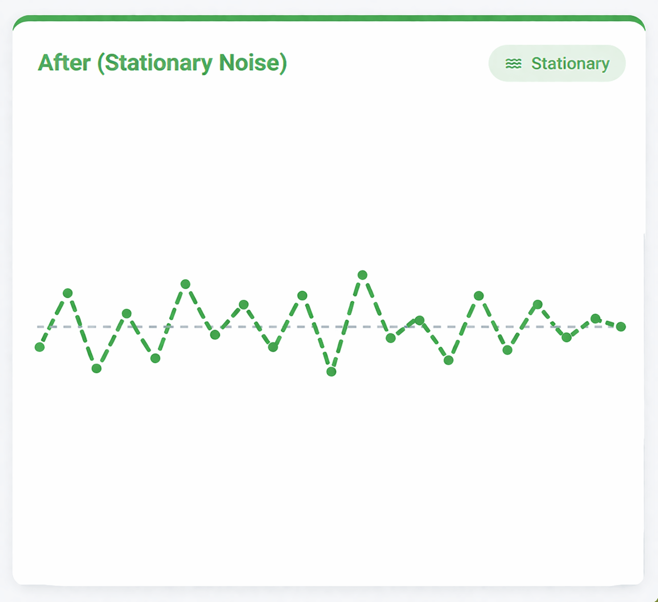
Apply seasonal differencing to time series data
1
Understand how SARIMA extends ARIMA for seasonal data
Standard ARIMA
Handled the Trend
Handled the Noise
Struggled with:
Repeating Pattern (Seasonality)
The Seasonal Upgrade
Now we capture the
Cyclical Seasonality
that repeats over time.
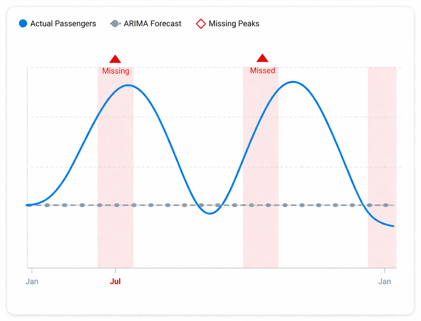
Forecasting Failure
The Problem:
Standard ARIMA draws a straight line into the future.
It completely ignores the repeating summer travel spikes.
Business Impact:
To schedule staff and set ticket prices, the airline must predict those peaks.
We need a model that understands seasons
Implemented in the statsmodels library
Standard ARIMA
p d q
Seasonal Blocks
P D Q s
SARIMAX
Complete Seasonal Model
from statsmodels.tsa.statespace.sarimax import SARIMAX
# We ignore the "X" for now
order = (p,d,q)
Controls the non-seasonal components (Trend, Lag, Noise).
seasonal_order = (P,D,Q,s)
Controls the seasonal components (Repeating cycles).
+
=
Monthly Data
Yearly patterns repeating every 12 months
Quarterly Data
Financial reports repeating every quarter
Daily Data
Website traffic patterns repeating weekly
Seasonal Period
Step: Seasonal Differecing
seasonal_diff = series.diff(12).dropna()
# subtracts this month from last year
Step: Building the Model
from statsmodels.tsa.statespace.sarimax import SARIMAX

model = SARIMAX(series,
                order=(1, 1, 1),
                seasonal_order=(1, 1, 1, 12))
results = model.fit()
Manual Code
Standard Order
order = (1,1,1)
Handles the baseline non-seasonal components (p, d, q)
Seasonal Order
seasonal_order = (1,1,1,12)
This is the crucial part that captures the annual repeating patterns.
Step: The Industry Short-Cut
import pmdarima as pm
model = pm.auto_arima(series, seasonal=True, m=12) # m is the same as s
1. Raw Data
Complex Seasonal Patterns & Unknown Parameters
2. Auto-ARIMA
Grid Search & Optimization
3. Optimal Result
Best (p,d,q) & (P,D,Q,s) found automatically
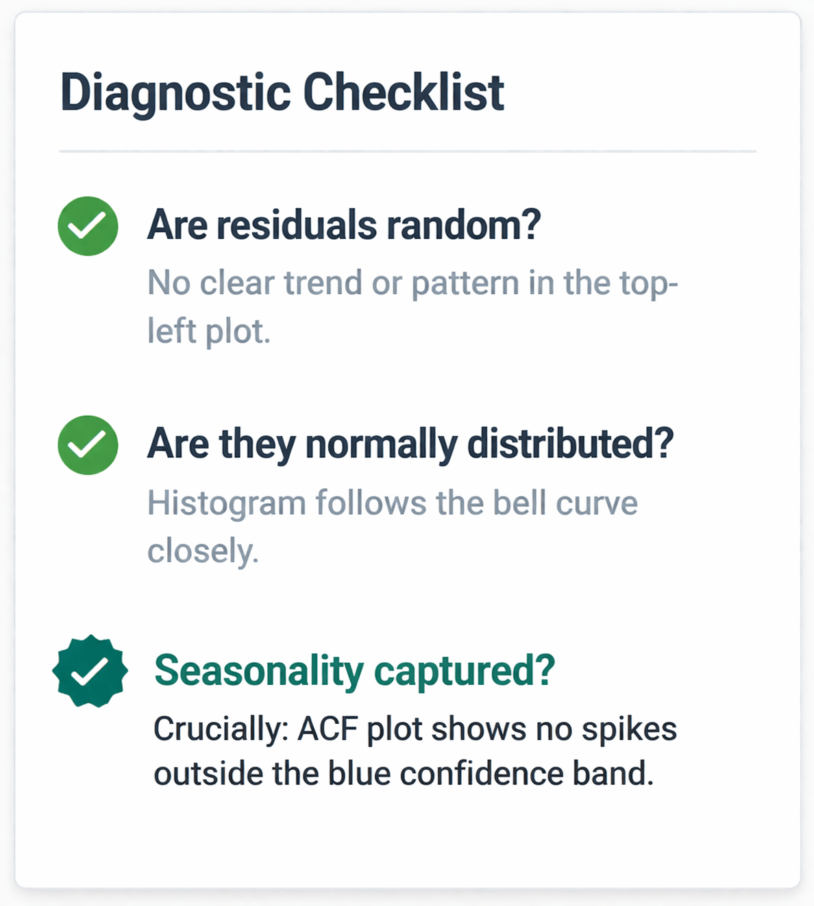
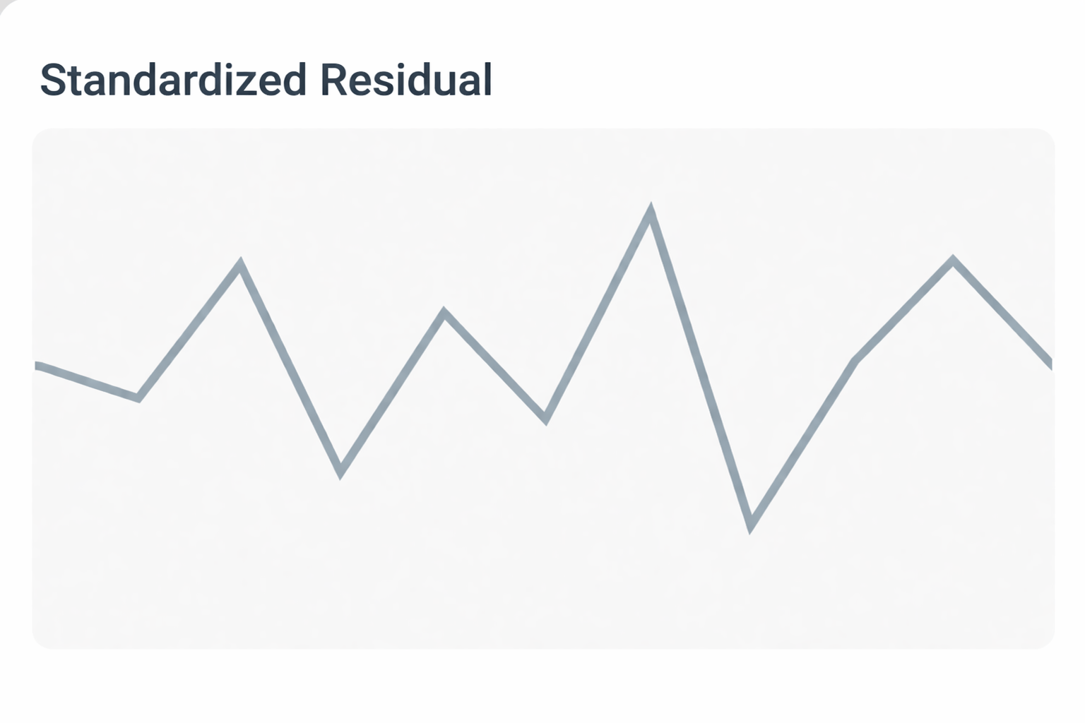
Step: Diagnostics
Are residuals random?
No clear trend or pattern in the top-left plot.
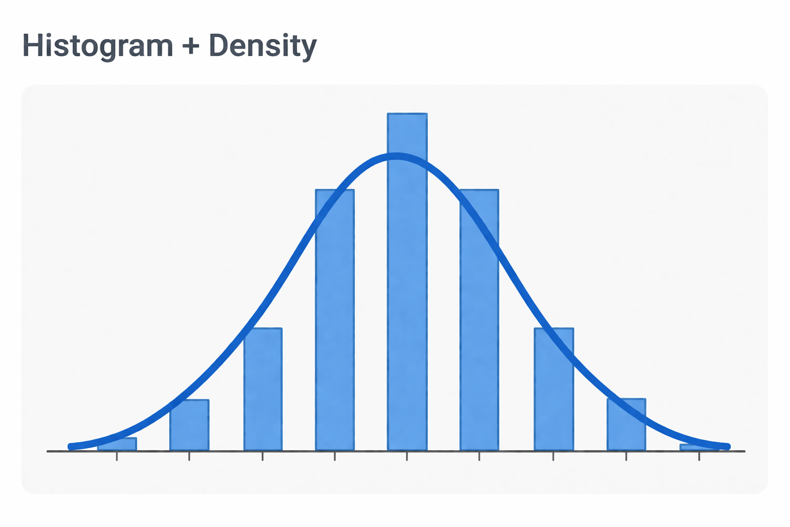
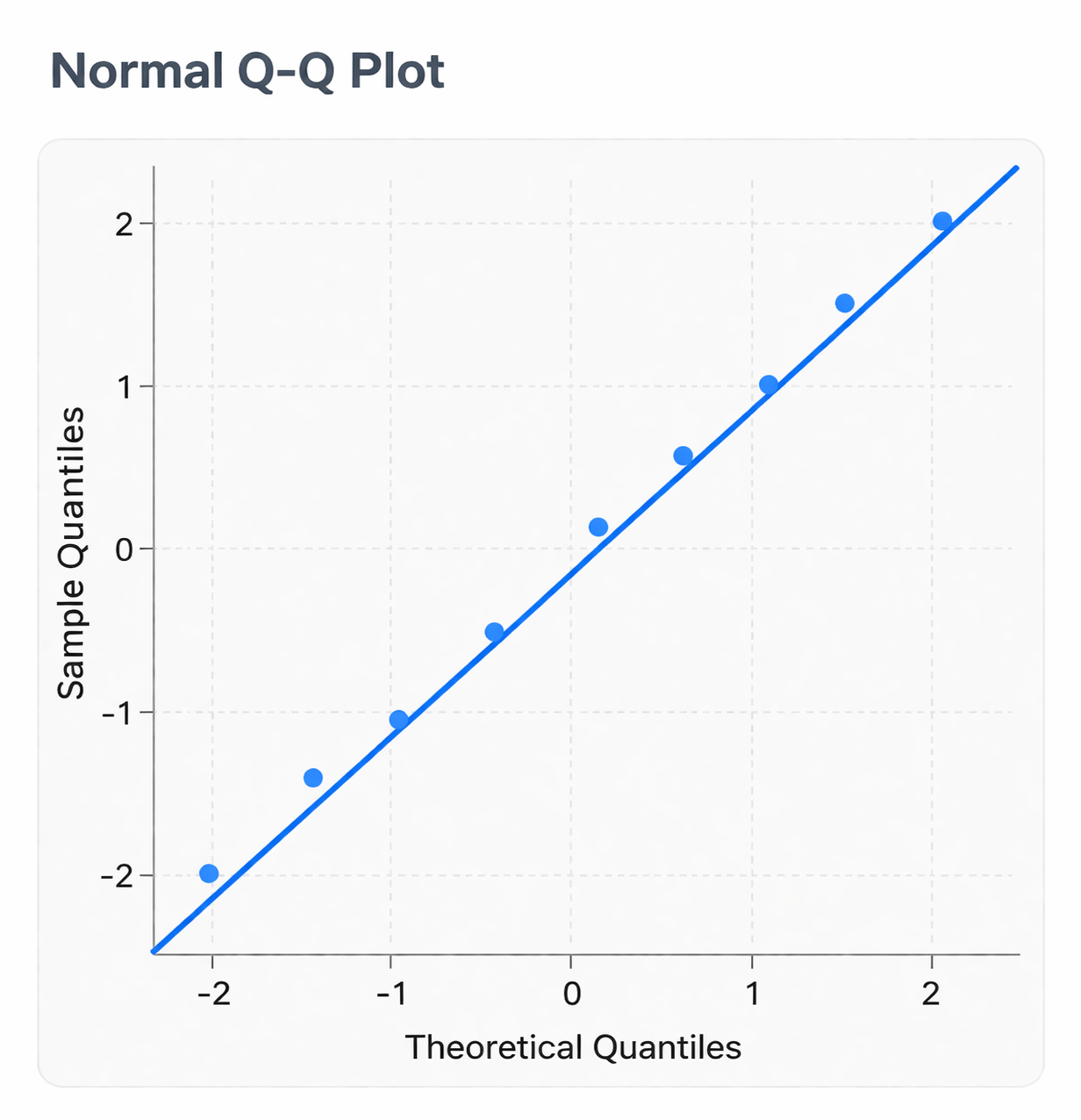
Are they normally distributed?
Histogram follows the bell curve closely.
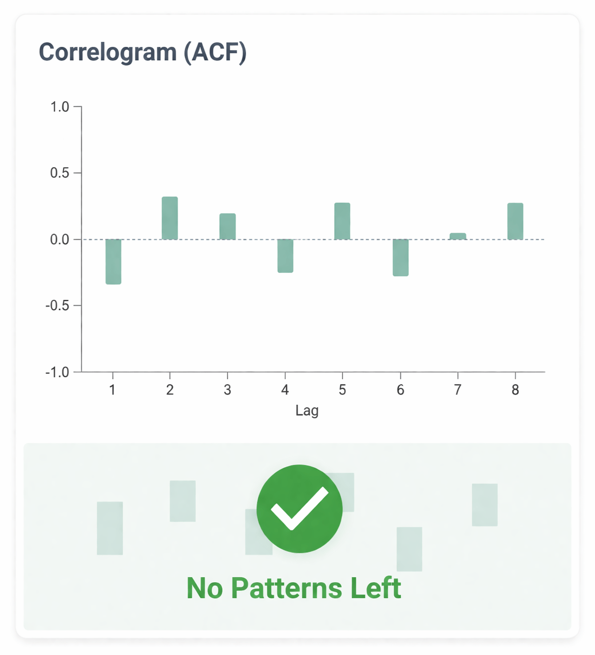
Seasonality captured?
Crucially: ACF plot shows no spikes outside the blue confidence band.
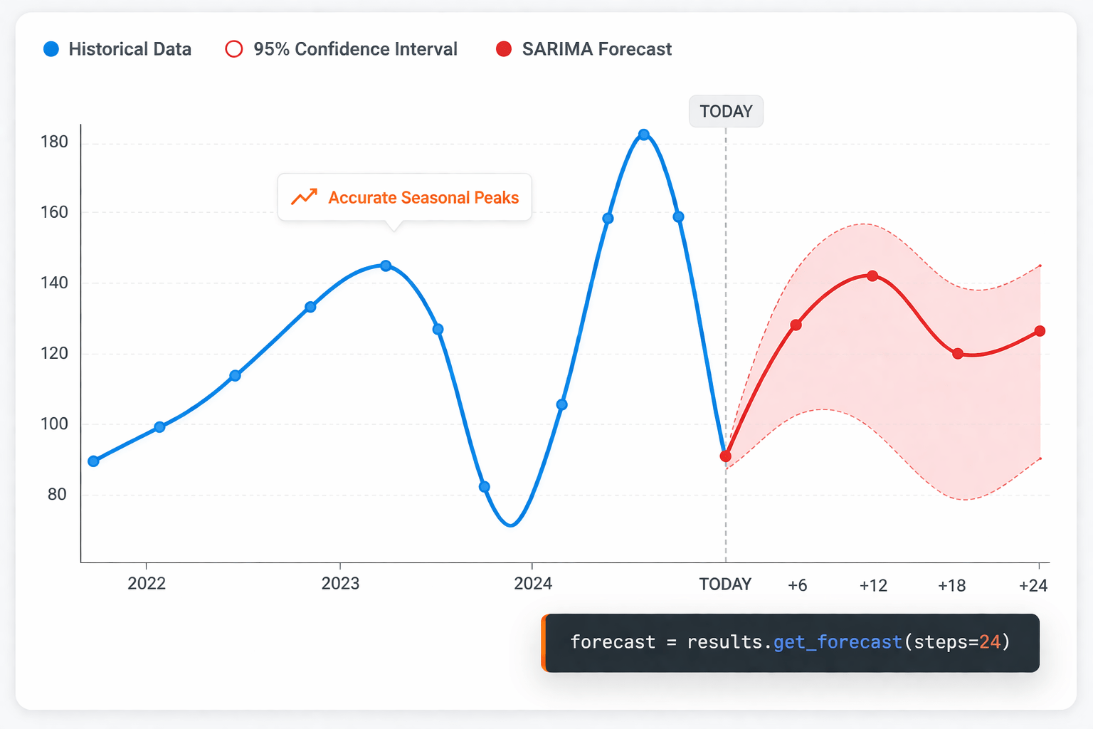
Step: Forecasting the Future
Summary
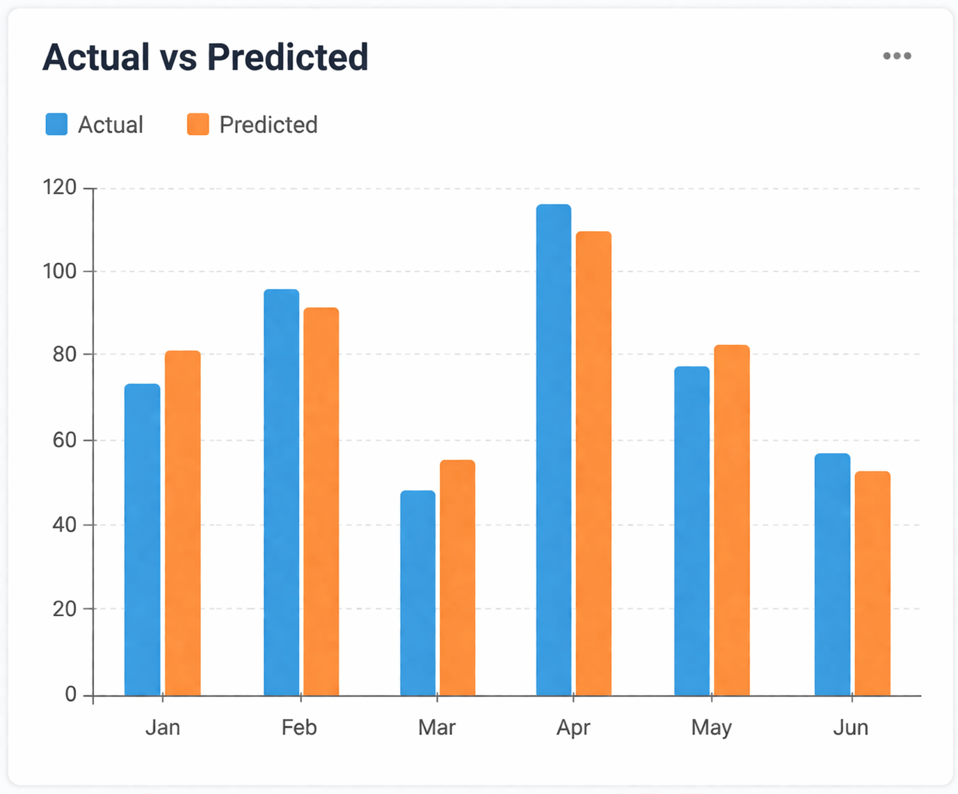
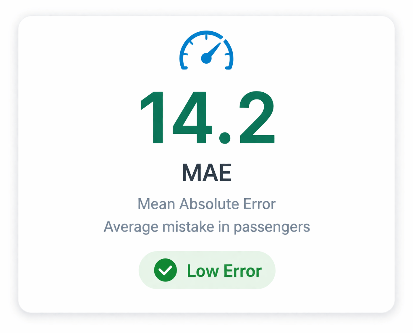
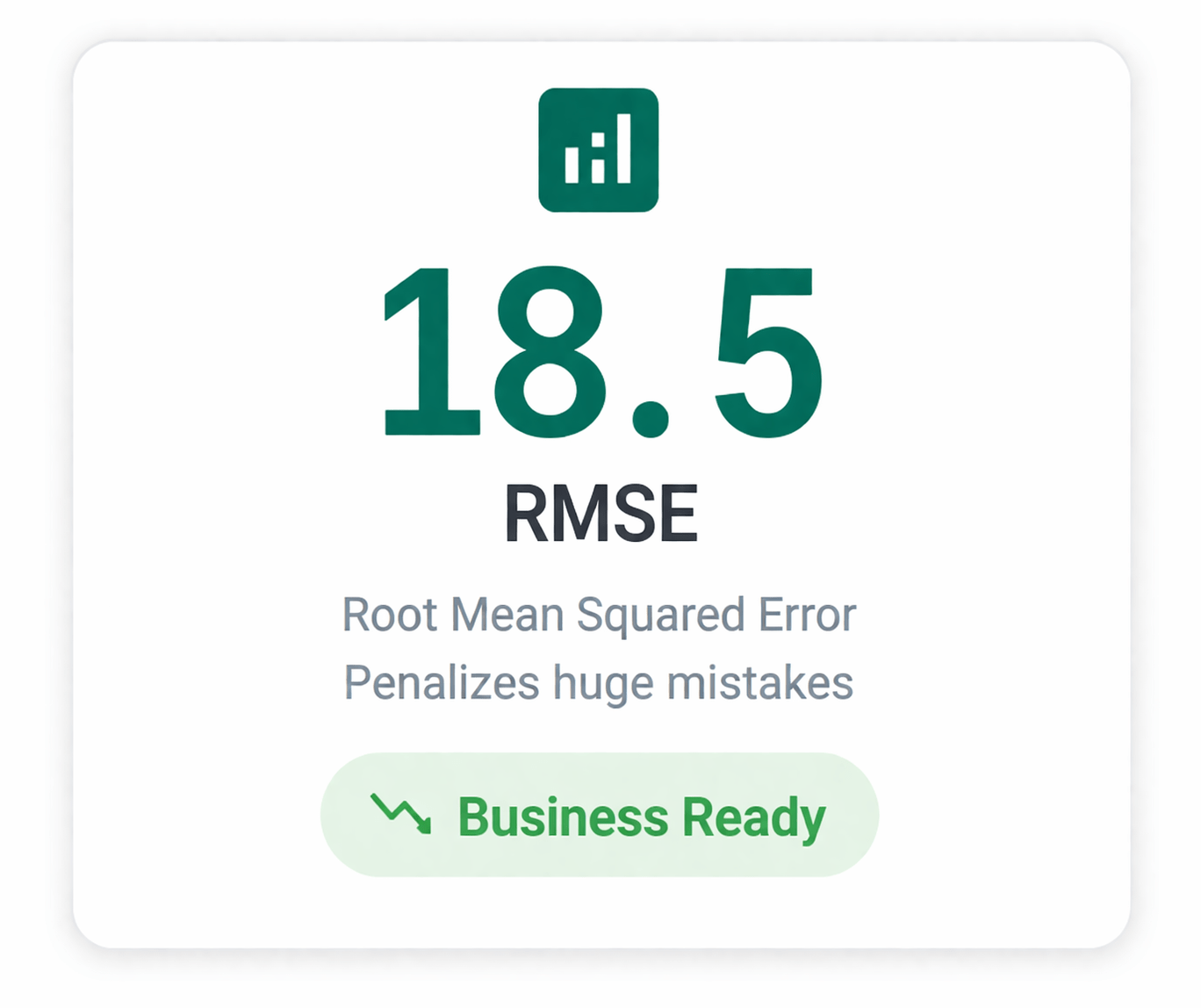
5
Forecast future values and measure accuracy (MAE/RMSE).
4
Check Residual Diagnostics to ensure no patterns were missed.
3
Fit the SARIMAX model.
2
Use auto_arima(seasonal=True) to find the best parameters.
1
Load Data & Identify Seasonal Period (s or m).
Quiz
When using auto_arima for monthly data with a yearly repeating pattern, what should the seasonal period parameter (m) be set to?
A. 1
B. 4
C. 7
D. 12
Quiz-Answer
When using auto_arima for monthly data with a yearly repeating pattern, what should the seasonal period parameter (m) be set to?
A. 1
B. 4
C. 7
D. 12
By Content ITV


