


Content ITV PRO
This is Itvedant Content department
Learning Outcome
4
Prepare analytically justified datasets for visualization
3
Interpret analytical results correctly
2
Apply these concepts using Pandas
1
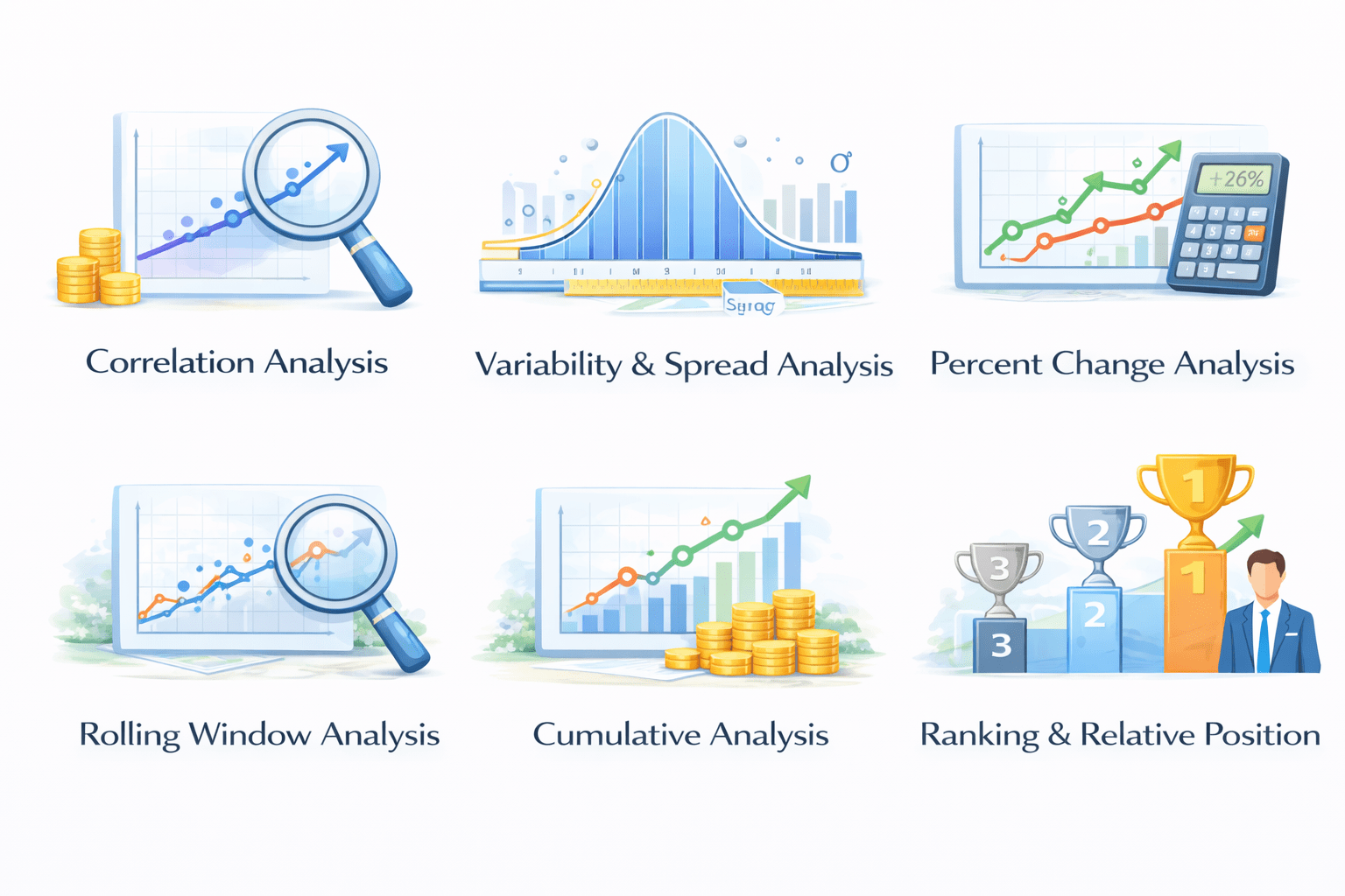
key analytical concepts such as correlation, rolling, and cumulative analysis
Clean, structured datasets
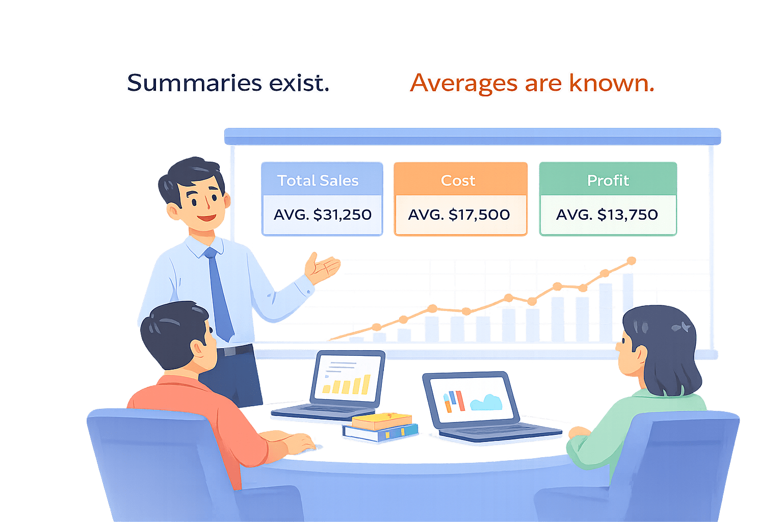
Aggregated summaries
Outputs from groupby() and pivot tables
Filtering and Sorting
Learners should know :
This topic focuses on analysis beyond summarization.
Imagine You made dashboard
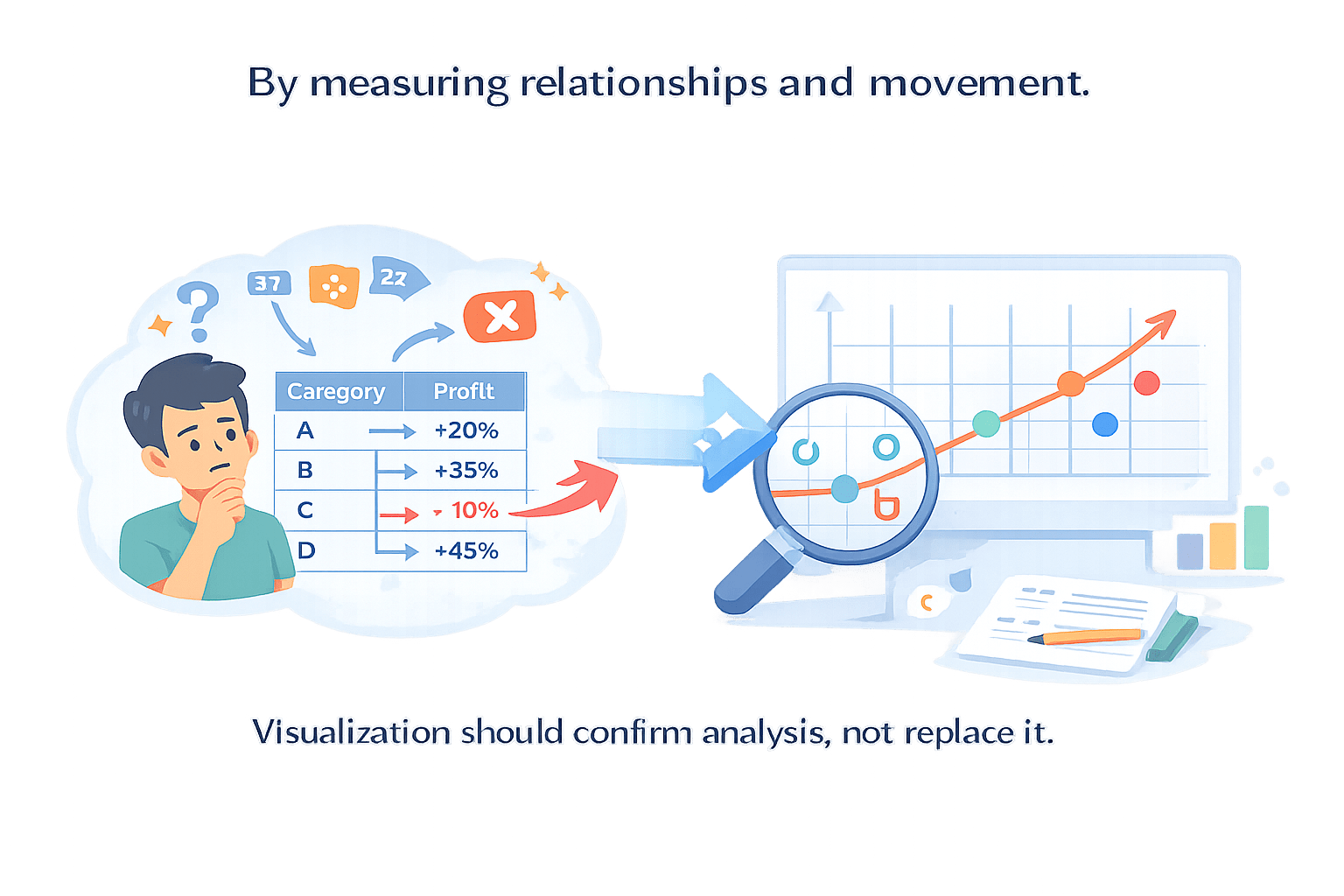
By measuring relationships and movement.
Visualization should confirm analysis, not replace it.
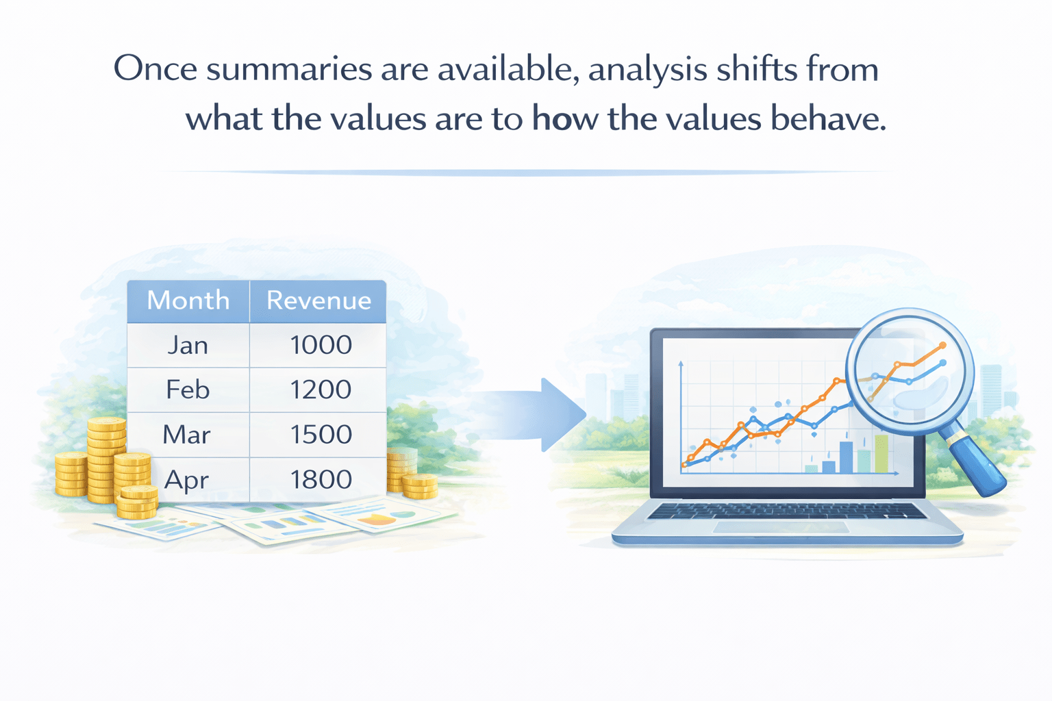
To see how this value behave we use following process
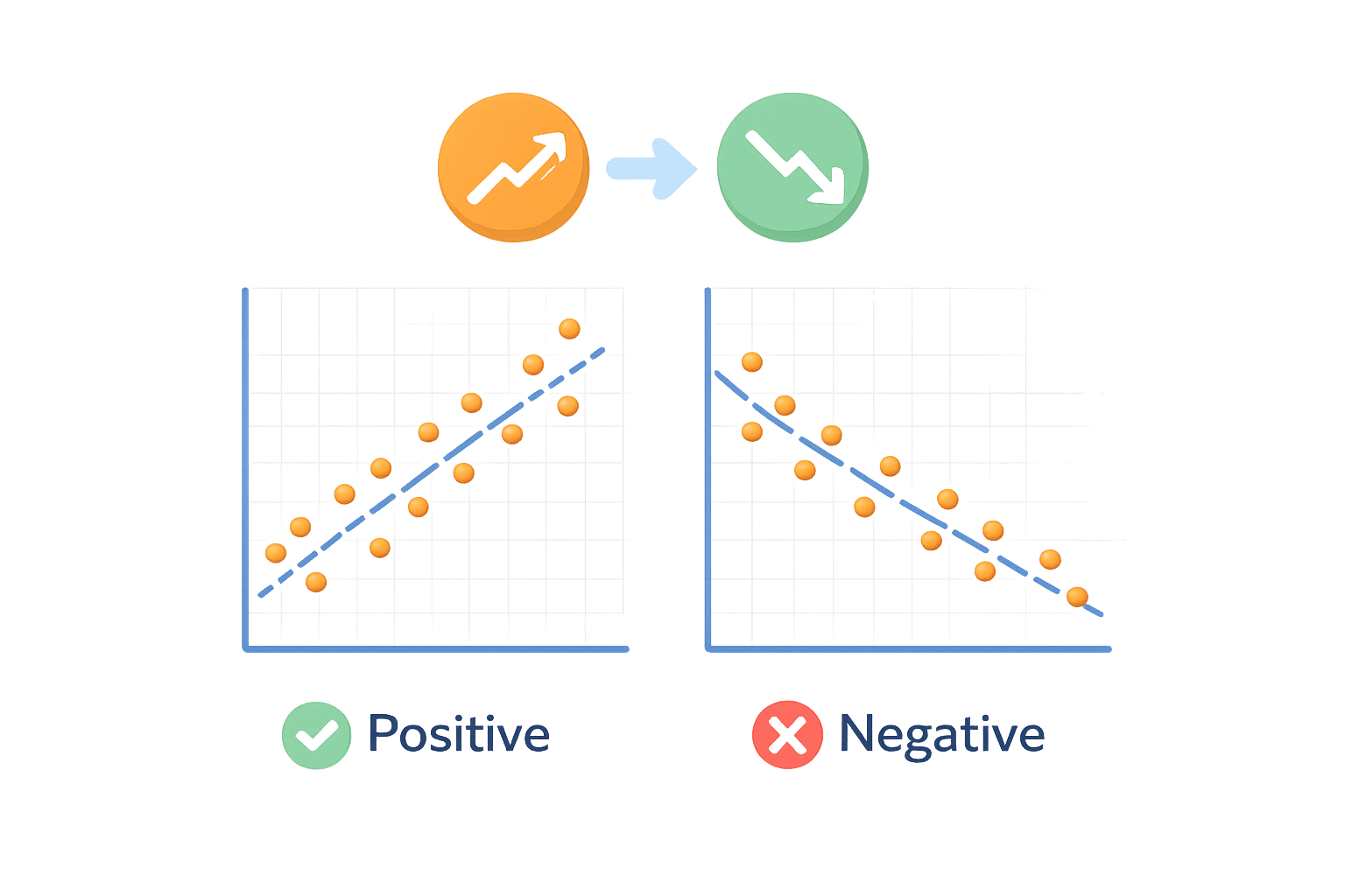
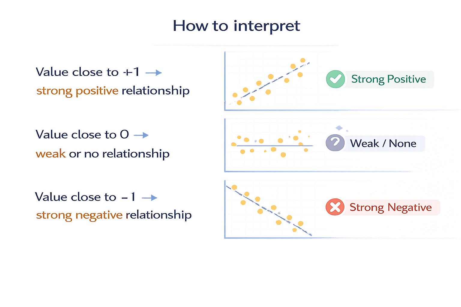
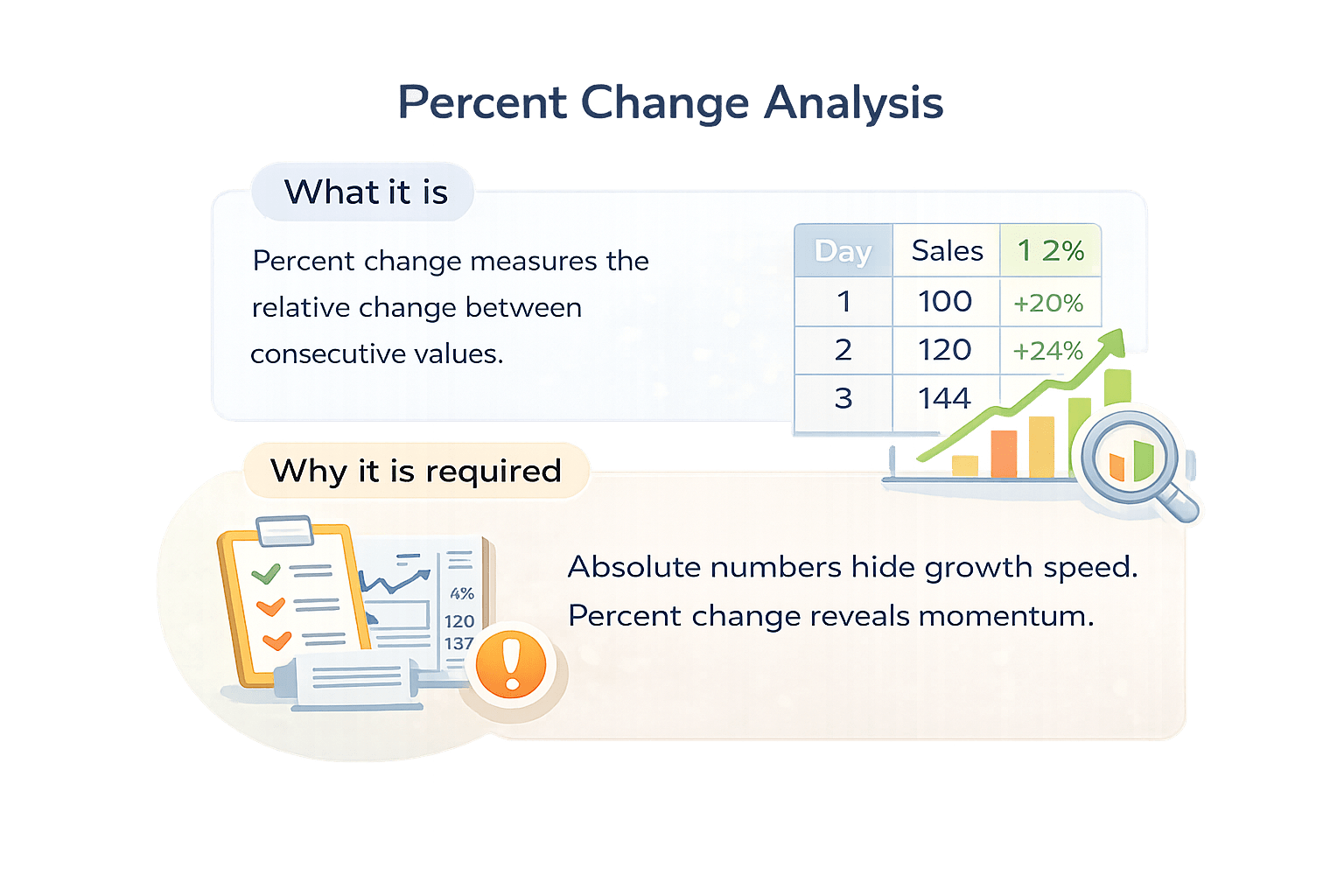
Correlation measures the strength and direction of a linear relationship between two numerical variables.
In simple terms:
When one value changes, does the other also change — and how strongly?
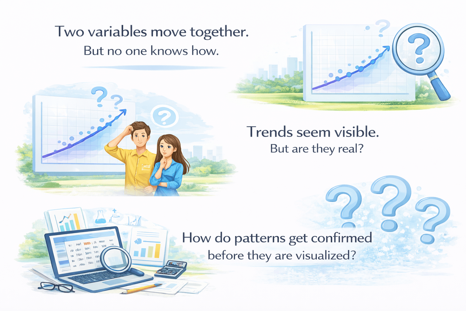
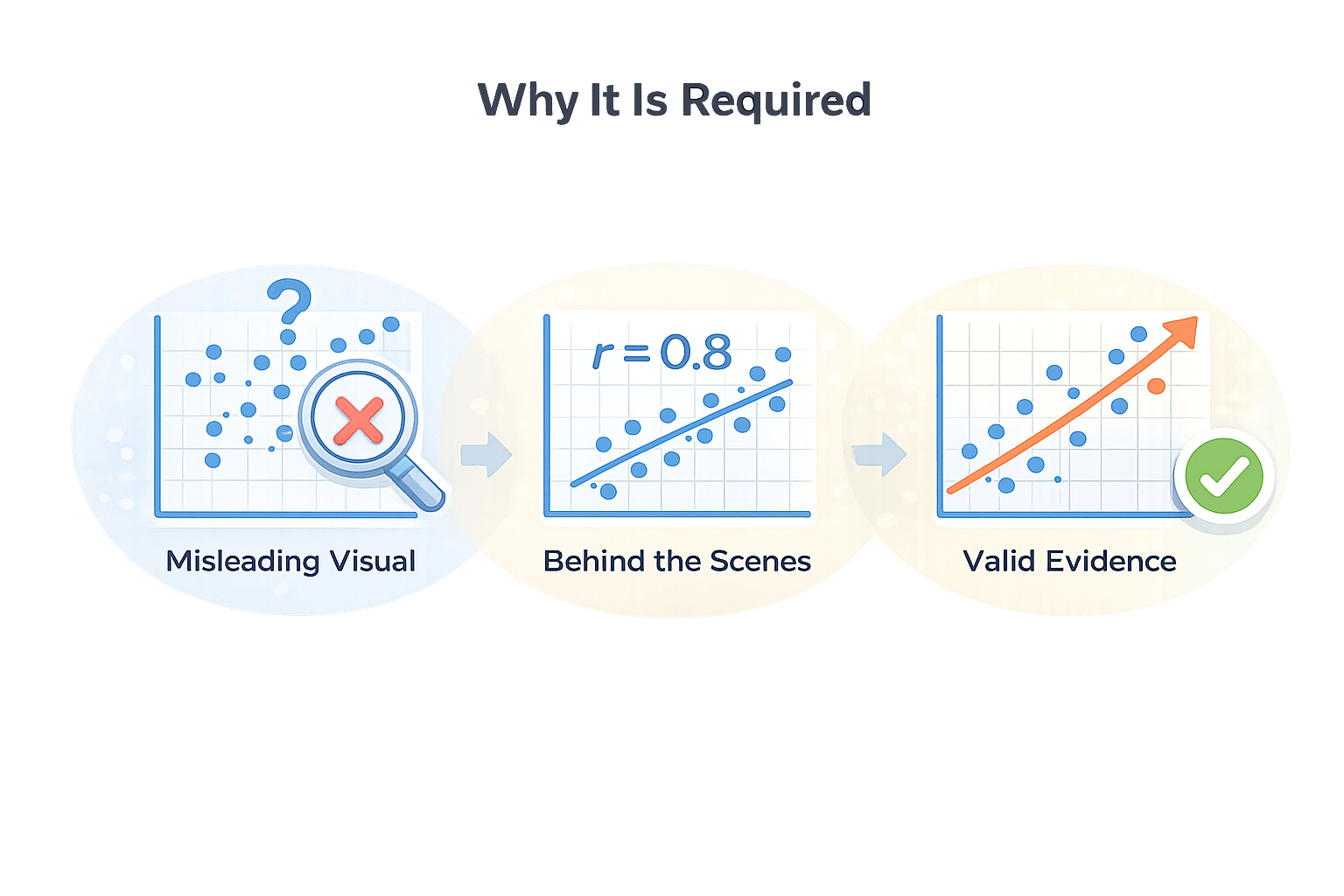
Visual inspection can be misleading.
Correlation provides numerical confirmation of relationships before visualization.
Why It Is Required
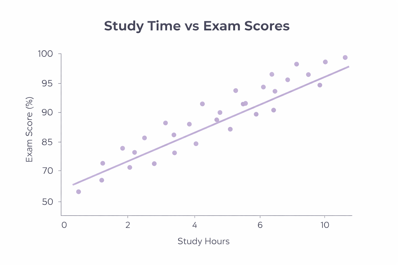
Imagine A teacher wants to understand:
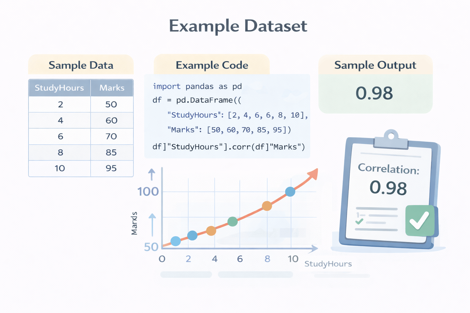
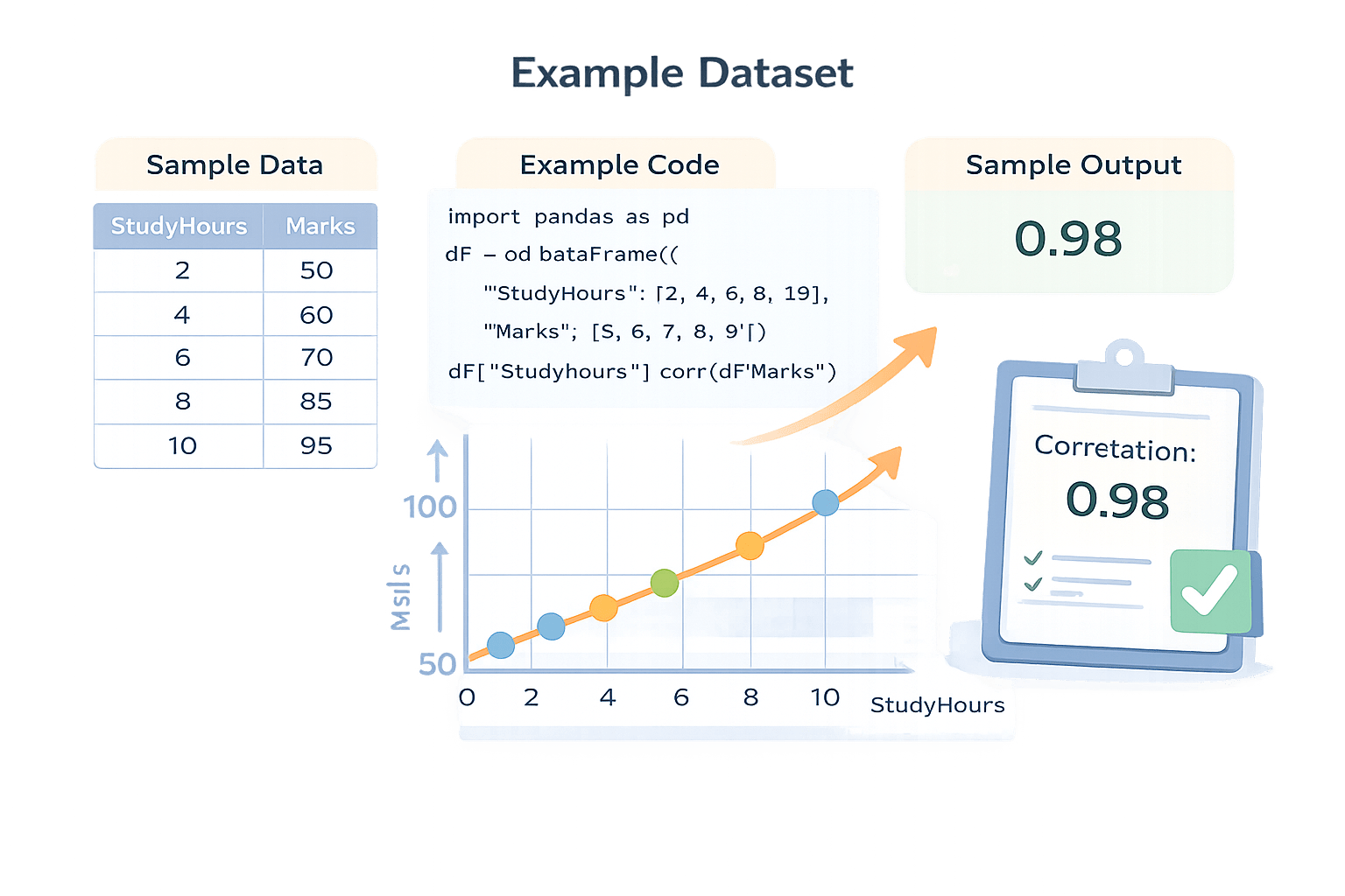
Does studying more hours actually lead to better marks?
In this scatter plot, every single point represents one student
import pandas as pd

df = pd.DataFrame({
    "StudyHours": [2, 4, 6, 8, 10],
    "Marks": [50, 60, 70, 85, 95]
})
Marks
Study Hours
df["StudyHours"].corr(df["Marks"])Output:
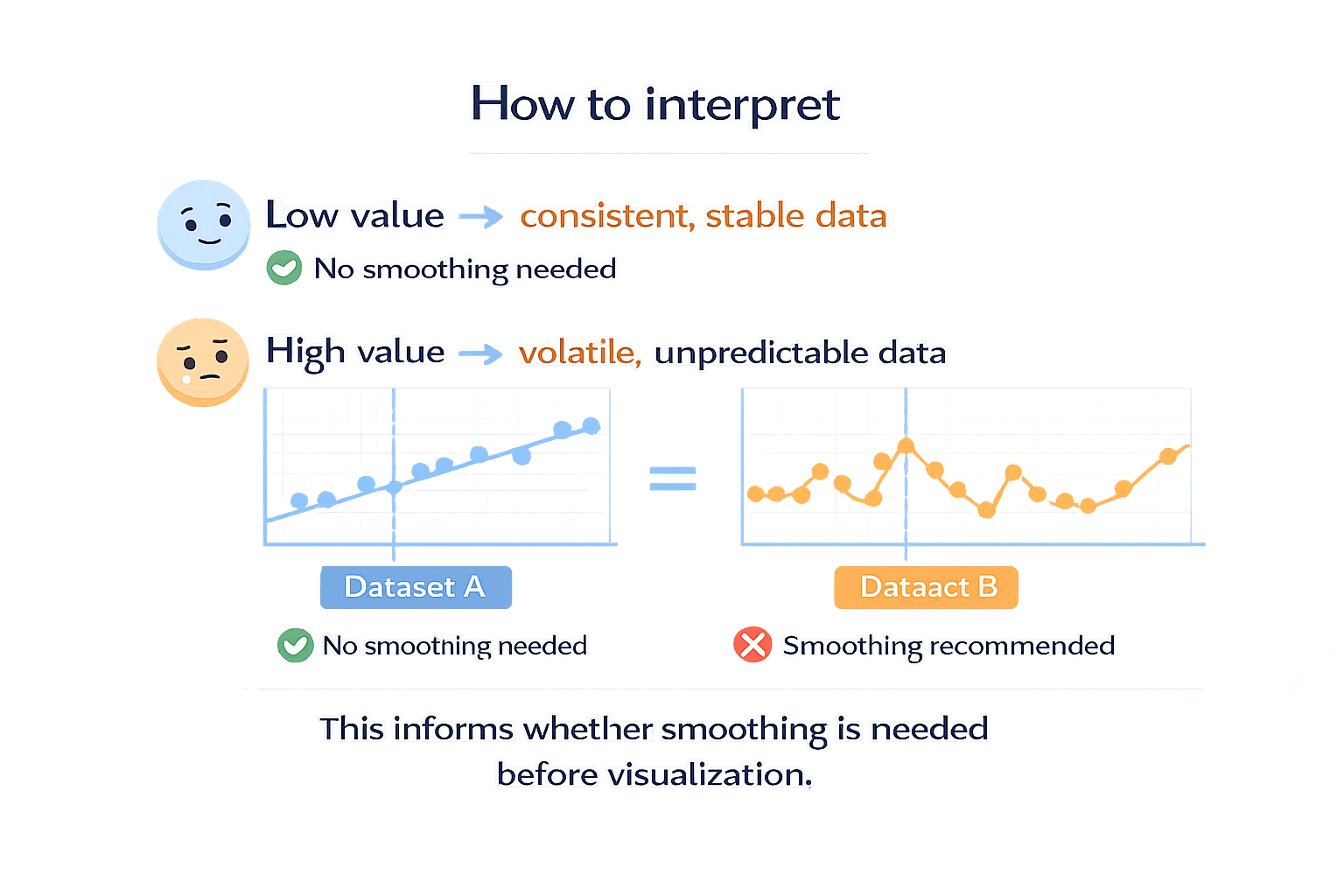
0.98How to Interpret
Variability and Spread Analysis
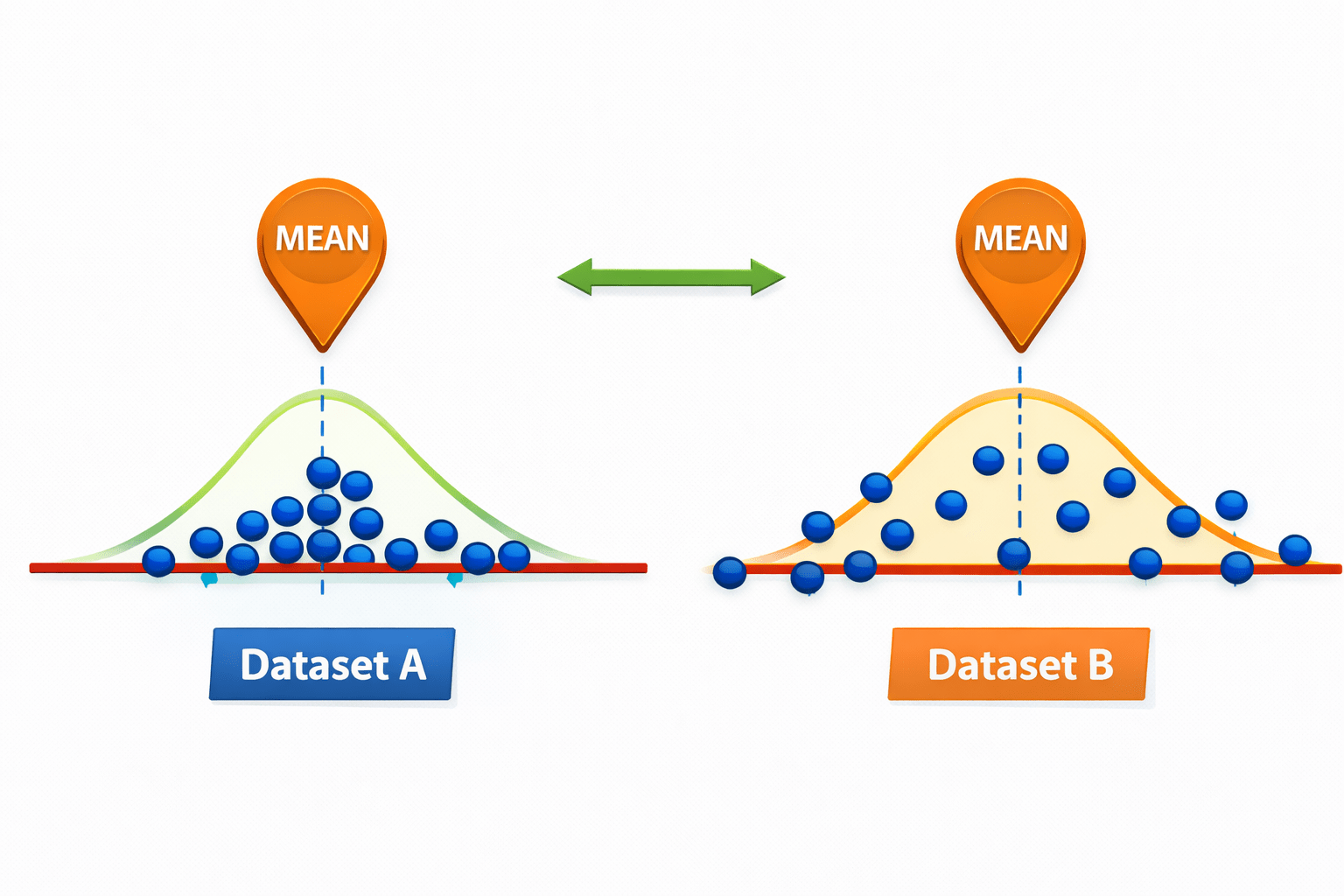
Variability describes how much values differ from each other, even if their average is the same.
Why it is required
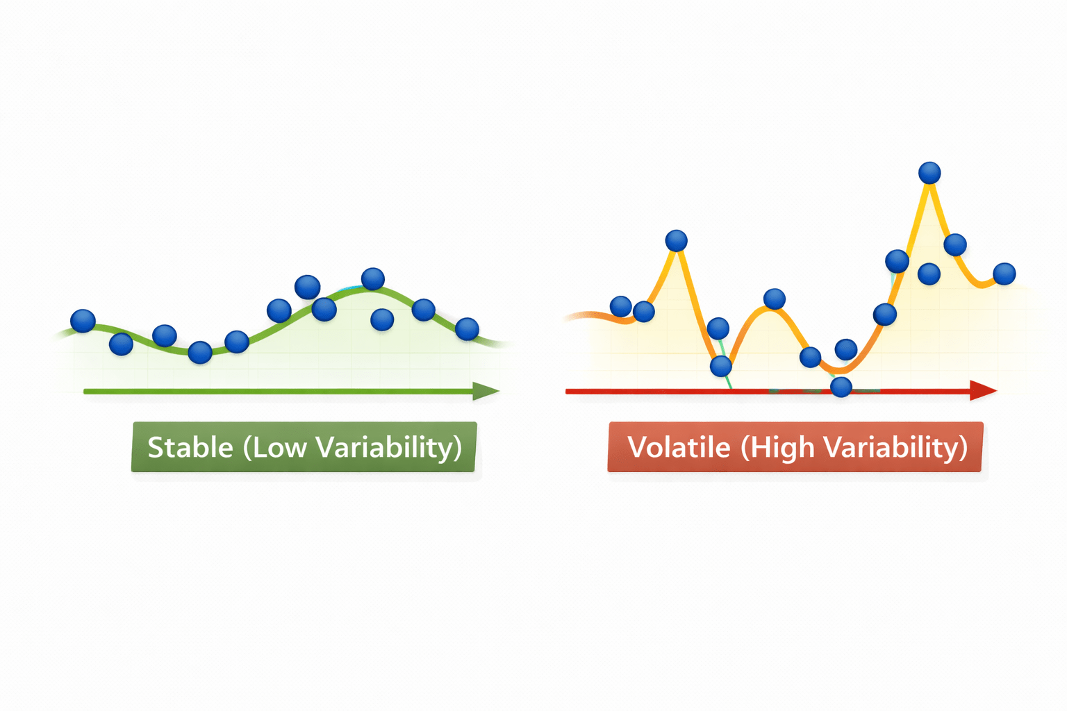
Two datasets can have the same mean but behave very differently.
Variability explains stability vs volatility.
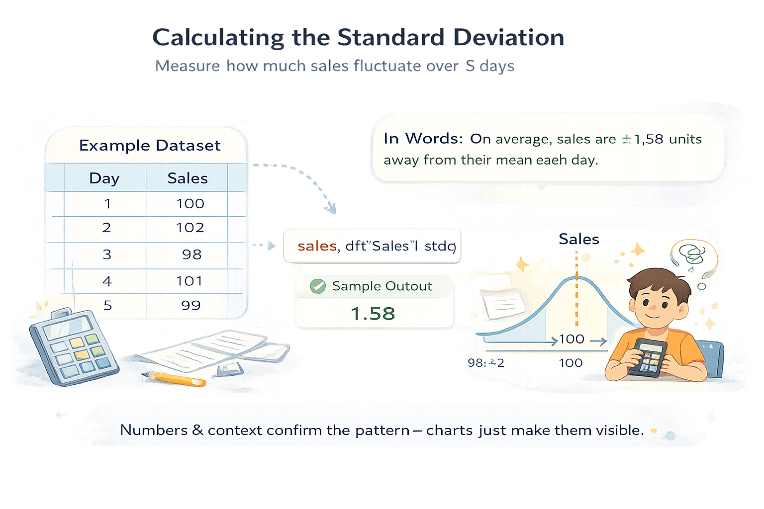
sales_df = pd.DataFrame({
    "Day": [1, 2, 3, 4, 5],
    "Sales": [100, 102, 98, 101, 99]
})
Imagime A small retail store tracks its daily sales for one working week to understand short-term behavior.
sales_df["Sales"].std()Output:
1.58Dataset B
Dataset A
Percent Change Analysis
+20%
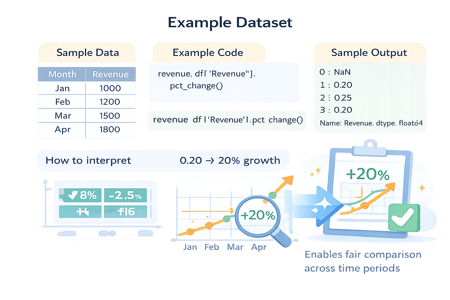
Imagine A startup tracks its monthly revenue for the first four months of the year to understand how the business is performing.
revenue_df = pd.DataFrame({
    "Month": ["Jan", "Feb", "Mar", "Apr"],
    "Revenue": [1000, 1200, 1500, 1800]
})
revenue_df["Revenue"].pct_change()0 NaN
1 0.20
2 0.25
3 0.20
Name: Revenue, dtype: float640 NaN
1 0.20
2 0.25
3 0.20
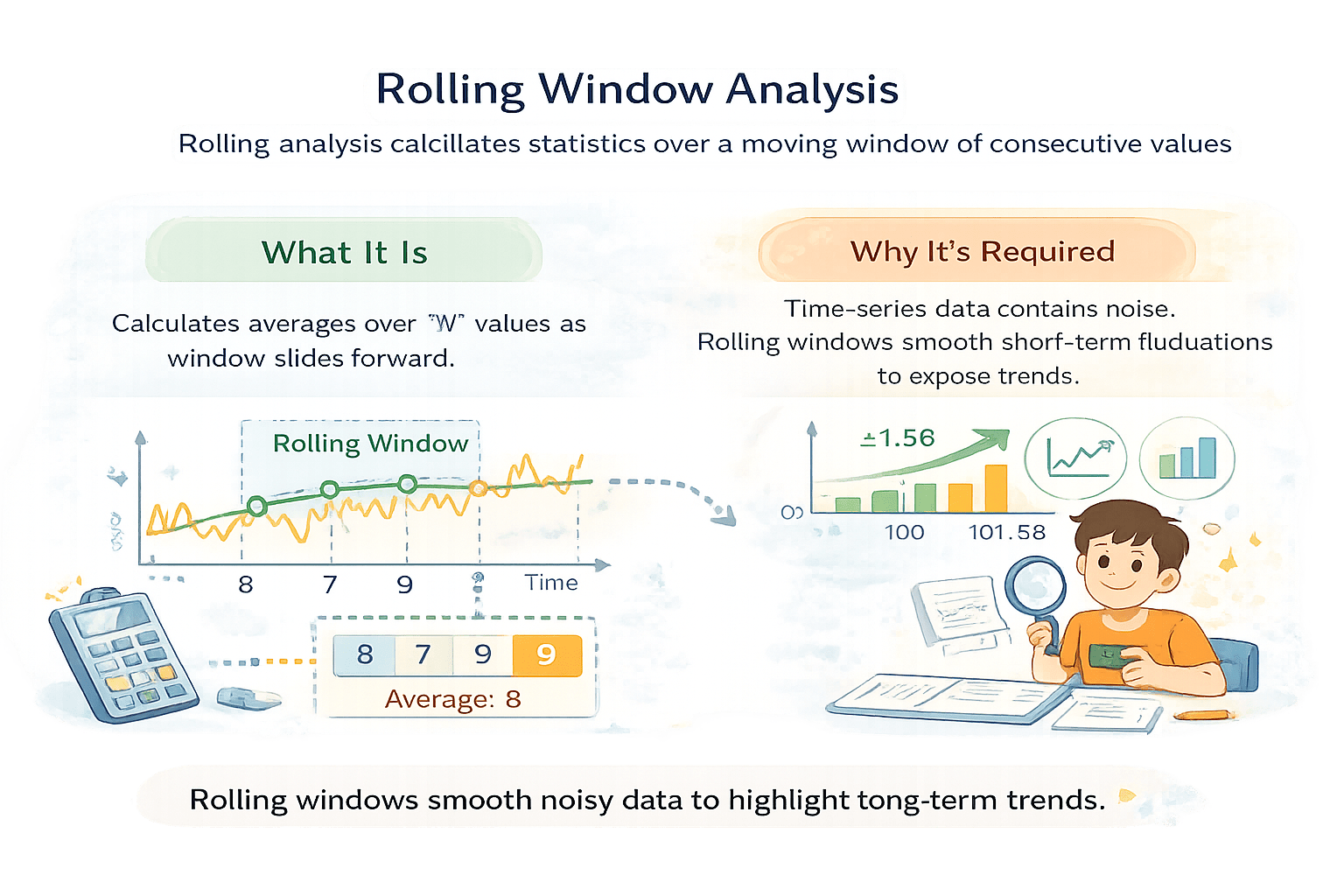
Name: Revenue, dtype: float64Rolling Window Analysis
Rolling analysis calculates statistics over a moving window of consecutive values.
Calculates averages over values as window slides forward
What It Is
8
8
Time-series data contains noise.
Rolling windows smooth short-term fluctuations to expose trends.
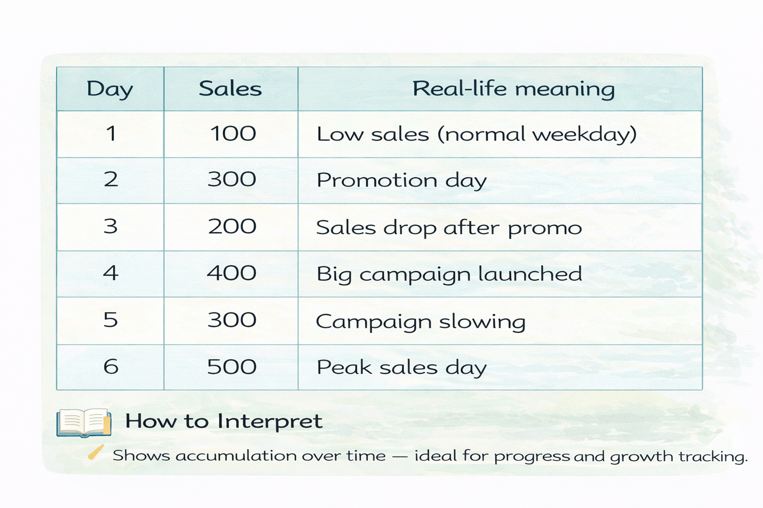
daily_sales = pd.DataFrame({
    "Day": [1, 2, 3, 4, 5, 6],
    "Sales": [100, 300, 200, 400, 300, 500]
})daily_sales["Sales"].rolling(window=3).mean()Imagine you run an online store.
Every day, sales fluctuate because of:
Discounts
Marketing campaigns
Weekends vs weekdays
Customer behavior
So daily sales are noisy and hard to judge by looking at single days.
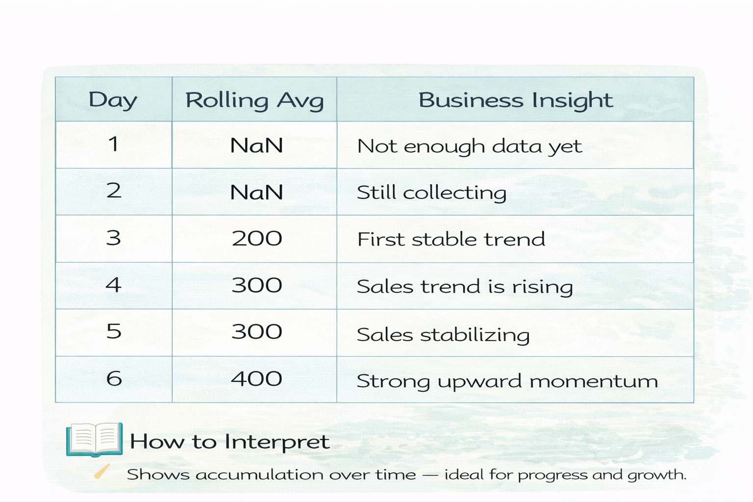
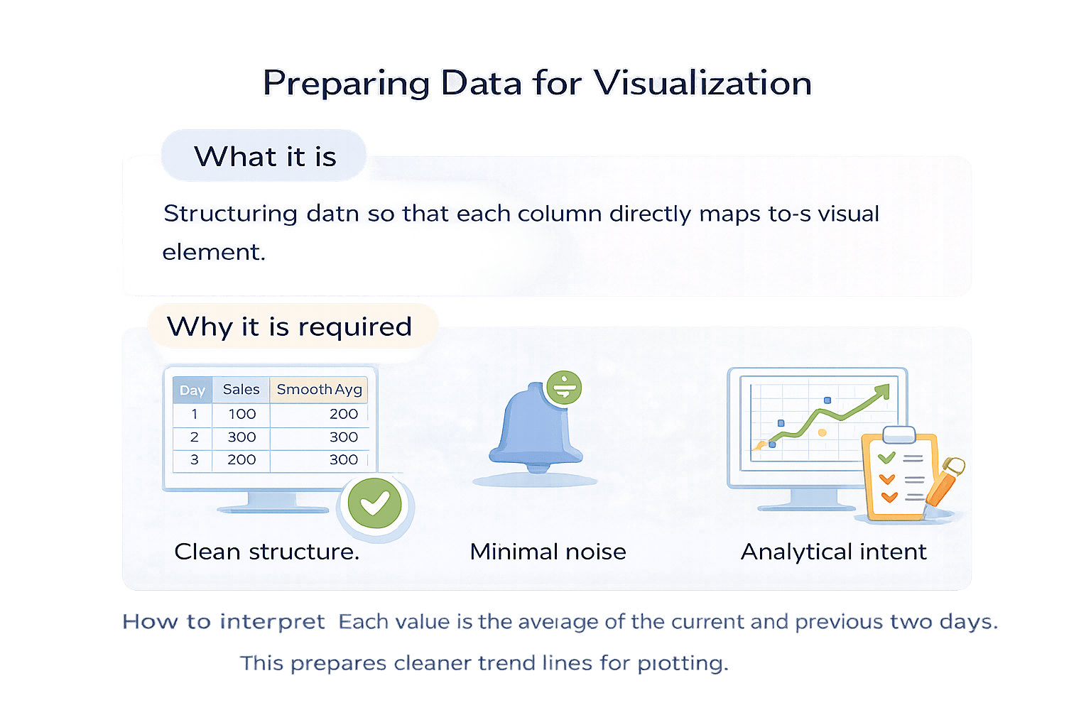
daily_sales["Sales"].rolling(window=3).mean()Rolling Average Interpretation (Window = 3)
Each value is the average of the current and previous two days.
This prepares cleaner trend lines for plotting.
How to interpret
Cumulative Analysis
401
500
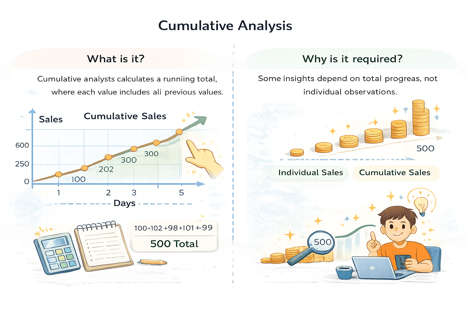
Cumulative analysis calculates a running total, where each value includes all previous values.
400
500
Some insights depend on total progress, not individual observations.
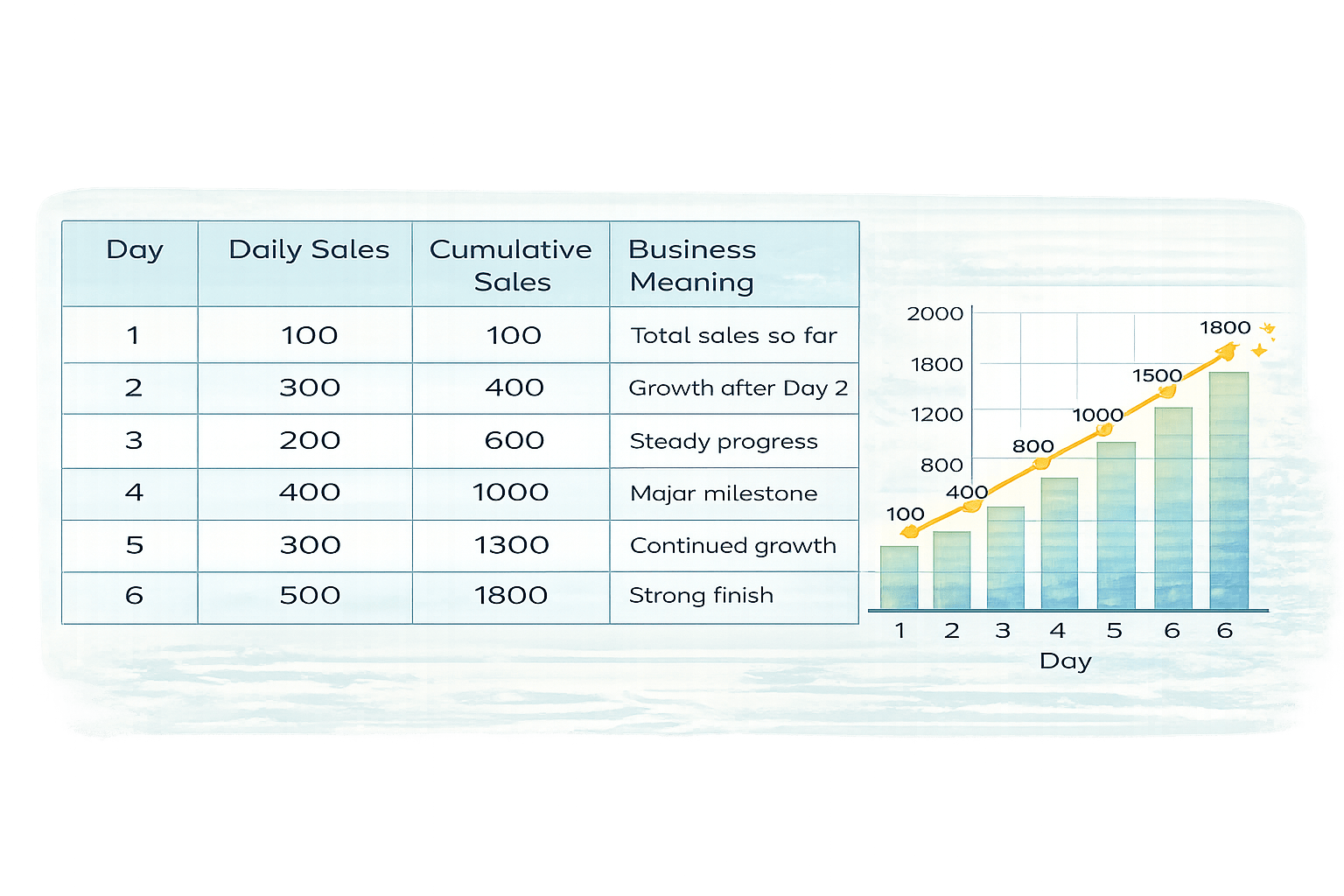
daily_sales["Sales"].cumsum()You own an online store and want to know:
daily_sales = pd.DataFrame({
    "Day": [1, 2, 3, 4, 5, 6],
    "Sales": [100, 300, 200, 400, 300, 500]
})
“How much total revenue have we generated so far each day?”
Daily sales fluctuate, but management cares about total progress, not just individual days.
That’s where cumulative analysis is used.
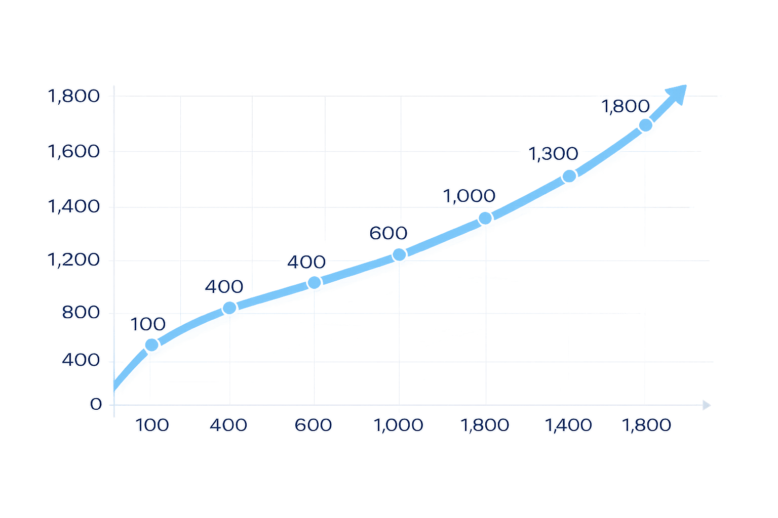
daily_sales["Sales"].cumsum()600
1300
1000
1800
2500
2000
1300
700
300
50
1
2
3
4
5
6
Day
Daily sales
Daily sales go up and down
Cumulative sales always increase
Shows overall business growth
How to interpret
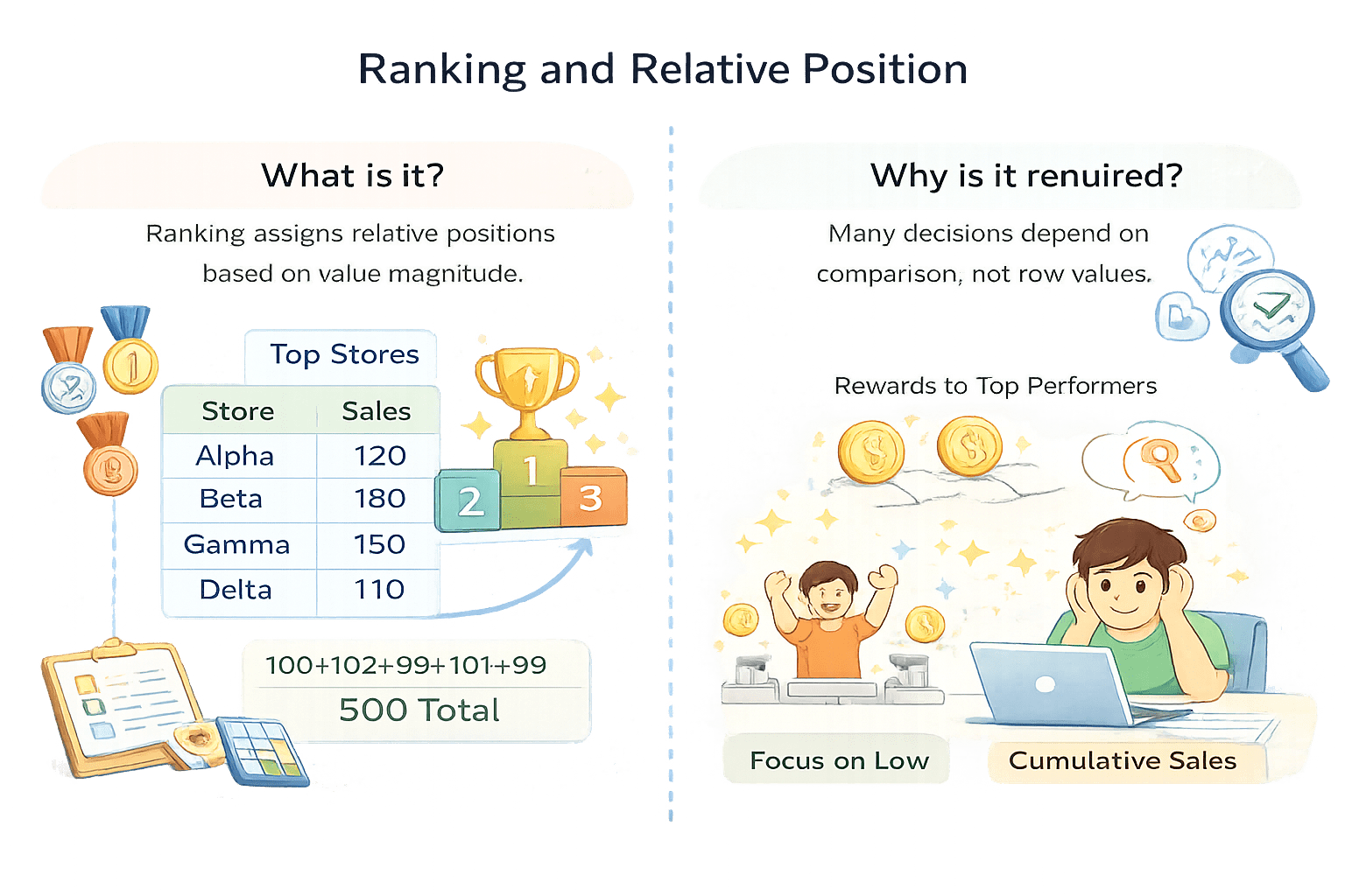
Ranking and Relative Position
What it is
Ranking assigns relative positions based on value magnitude.
Why it is required
Many decisions depend on comparison, not raw values.
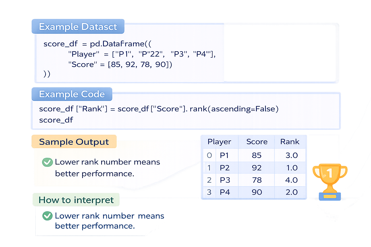
score_df = pd.DataFrame({
    "Player": ["P1", "P2", "P3", "P4"],
    "Score": [85, 92, 78, 90]
})
score_df["Rank"] = score_df["Score"].rank(ascending=False)
score_dfImagine a school sports tournament
where players earn points based on their performance in matches.
Preparing Data for Visualization
Structuring data so that each column directly maps to a visual element.
smooth Avg
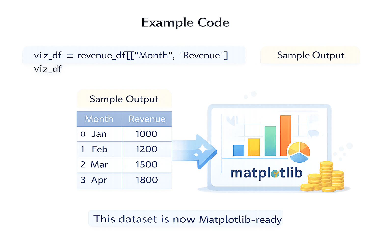
revenue_df = pd.DataFrame({
    "Month": ["Jan", "Feb", "Mar", "Apr"],
    "Revenue": [1000, 1200, 1500, 1800]
})

viz_df = revenue_df[["Month", "Revenue"]]
viz_df
This Dataset is now Matplotlib - ready
Imagine you have some Data
Summary
5
Ranking enables comparison
4
Cumulative analysis shows progress
3
Rolling analysis reveals trends
2
Variability explains stability
1
Correlation measures relationships
Quiz
What does rolling analysis help identify?
A. Exact totals
B. Short-term noise
C. Long-term trends
D. Data types
What does rolling analysis help identify?
A. Exact totals
B. Short-term noise
C. Long-term trends
D. Data types
Quiz-Answer
By Content ITV


